Rarely categorical, highly separable representations along the cortical hierarchy - Nature

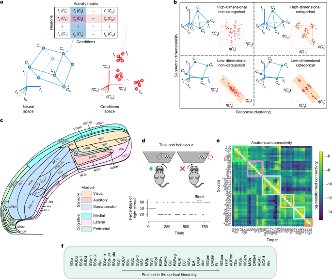
MainNeural responses are often complex, depend on multiple variables (mixed selectivity6) and, in cognitive areas, are very diverse and seemingly disorganized3,7,8. One of the challenges in neuroscience is finding meaningful structure in seemingly disorganized data. This structure has traditionally been investigated in single-neuron responses by looking for easily interpretable tuning curves (for example, orientation selectivity in visual cortex or place cells in the hippocampus). When considering a large number of neurons, interesting structures are emerging, both in the statistics of the responses of individual neurons and at the level of population responses. Here we focused on both types of structure, how they are related to each other and what computational implications they entail. Consider the neural activity estimated in one particular time interval, recorded in different experimental conditions (for example, in response to different sensory stimuli)3,9,10: the responses of the different recorded neurons can be organized into a matrix (Fig. 1a) in which each row represents the responses of a neuron to all of the experimental conditions. This matrix defines two complementary spaces: one spanned by the rows, indexed by condition number, called the conditions space (Fig. 1a (red)), and the other spanned by its columns, indexed by neuron number, called the neural space (Fig. 1a (blue)).Fig. 1: Conceptual framework and data structure.a, The matrix of neural responses of N neurons in M experimental conditions can be analysed in either its row space (conditions space, red) or column space (neural space, blue). The relative position of conditions in the neural space defines their representational geometry. If neurons are clustered in the conditions space, they define what is called a categorical representation1,2,3. b, The extent to which these two perspectives are related to each other is unclear, and neural populations could, in principle, occupy any portion of the clustering-dimensionality space. The image was adapted with permission from ref. 3, Elsevier. c, Swanson flat map of the 43 cortical regions that we analysed. Data were recorded by the IBL consortium (IBL Brainwide Map dataset) using Neuropixels probes. After selecting neurons in the cortex, we were left with around 14,000 neurons from around 180 recording sessions. d, In the IBL task, mice need to rotate a wheel to move a visual stimulus towards the centre of the screen. The stimulus appears left or right with an 80–20% biased probability in blocks of trials (bottom), adding prior contextual information to the task. The diagram was reproduced from refs. 4,50 under a CC BY 4.0 licence. e, Region-to-region anatomical connectivity in the cortex; data are from ref. 5. The coloured boxes highlight six anatomical modules with dense intramodule connectivity. f, Cortical hierarchy derived by the anatomical connectivity matrix of e. The order was derived previously5, such that source regions (that is, regions whose connectivity is unbalanced outwards) are mostly placed low, and target regions (that is, regions whose connectivity is unbalanced inwards) are mostly placed high in the hierarchy. Additional details on how the hierarchy is computed and definitions of cortical region abbreviations can be found in ref. 5.In the conditions space, each point represents the response profile of a single neuron to the experimental conditions. If groups of neurons respond similarly, they will form clusters (functional groups) in this space, defining what was previously1 called a categorical representation (Fig. 1a). Distinct clusters represent categories of neurons with specific functional properties. In non-categorical representations, neurons can exhibit diverse responses whose distributions do not cluster.Categorical representations have been reported in the orbitofrontal cortex of rodents2,11 and monkeys12, whereas non-categorical representations were found in the rodent posterior parietal cortex1 and in reward-sensitive frontostriatal brain areas in monkeys performing a variety of economic decision-making tasks13. In several other articles6,14,15,16,17, the authors did not examine whether the representations are categorical, but the observation of diverse mixed-selectivity neurons and high-dimensional representations suggests non-categorical representations (Discussion). Whether, where and how neural populations are subdivided into functional clusters is still an open debate3.In the space spanned by the columns of the matrix, each point represents the population response to one experimental condition. The set of distances between all pairs of points defines the geometry of the neural representations (Fig. 1a). Analysing this geometry has been shown to provide insights into the brain’s encoding strategies and their computational implications for learning and flexible behaviour6,15,16,17,18. For example, a high-dimensional neural geometry confers flexibility to a simple linear readout6,7,8, as the same representation can support a large number of different output functions. High-dimensional representations also maximize memory capacity16, whereas low dimensionality is associated with abstract representations and generalization in novel situations7,15,18. How the dimensionality of population activity in the neural space is related to the clustering of response profiles in the conditions space is still an open question (Fig. 1b).Here we systematically analysed the response profiles and the representational geometry of 14,000 neurons from 43 cortical regions (Fig. 1c) in mice performing a decision-making task (IBL public Brainwide Map dataset4; Fig. 1d) and related the functional properties of cortical areas with their anatomical properties as reported by the Allen Mouse Brain Connectivity Atlas5 (Fig. 1e,f). As neuronal responses exhibit complex temporal profiles, we applied a reduced-rank regression (RRR) model to characterize both the temporal and selectivity components of individual neuron response profiles. We found that the selectivity profiles within individual areas are clustered (that is, categorical) only in primary sensory areas. When multiple brain areas are considered, we observe clustering that reflects the brain’s large-scale organization. The response profiles of neurons in different brain regions differ enough that a decoder can determine the region to which a particular neuron belongs. Finally, we investigated the computational implications of the observed representations by studying the separability of the different experimental conditions, a measure of how many different classifications in the activity space can be solved by a linear readout6. Brain areas with more diverse neural responses (less structured) exhibit higher separability.Our results reveal a systematic relationship between clustering and representational geometry, providing a large-scale perspective on neural selectivity and population coding across the cortex.Response profiles of individual neuronsTo characterize the response profiles, we used a linear encoding model and, in particular, a RRR model that predicts the activity of single neurons in response to changes in a set of variables that characterize each experimental condition and the behaviour of the mouse (Fig. 2a). The core component of the RRR encoding model is a small set of temporal bases, learned from data and shared across neurons to describe their time-varying responses (see Extended Data Fig. 1 for a schematic of the RRR model and the Methods for its mathematical formulation and comparisons with previous regression models4,19,20). Sharing temporal bases substantially reduces the number of parameters and mitigates overfitting.Fig. 2: Large-scale functional organization of the cortex.a, Schematic of single-neuron selectivity estimation. A linear encoding model describes a neuron’s temporal responses as a function of task and behavioural variables. Selectivity (α) is the sum of coefficients over time. Relevant variables, neural activity, estimated coefficients and selectivity are shown for an example trial. b, The goodness of fit (threefold cross-validated R2) of our encoding model versus computing the PSTH per task condition. Inset: outperformance (ΔR2). c, Average (absolute) selectivity profiles for neurons in the analysed cortical areas, normalized per input variable (columns). The triangles mark the top three selective areas per variable. d, Correlation between region-to-region functional similarity (cosine similarity between the average selectivity profiles in c) and their anatomical connectivity from Fig. 1e. Each dot is a pair of cortical areas (Spearman correlation, ρ = 0.40, P = 1.8 × 10−10). e, Multiclass decoding performance of the region or module labels from the time-varying response profiles of individual neurons (regions: accuracy = 0.233; null = 0.033 ± 0.003; P ≈ 0; modules: accuracy = 0.422; null = 0.203 ± 0.010). Decoding performance is measured as the one-versus-one multiclass accuracy of a linear SVM. The error bars indicate the distribution of decoding performance after random label shuffling. Module labels are defined as shown in Fig. 1, following ref. 5. f, The binary region-to-region decoding performance is inversely correlated with the anatomical connectivity (from Fig. 1e) between the two regions involved (Spearman correlation ρ = −0.49, P = 3.7 × 10−14). g, Schematic of the independent conditions analysis. Conditions are defined by the largest set of combinations of motor, sensory and cognitive variables that are well represented in the behaviour. Bottom, an example of the number of trials per condition in a session. h, Two examples of geometries in the neural space with different numbers of independent conditions (MIC = 4, left; MIC = 2, right). i, The number of independent conditions increases along the hierarchy. The shaded areas in d, f and i indicate the bootstrap 95% confidence intervals of the fitted regression lines. P values for Spearman correlations were computed using SciPy’s two-sided test; ***P < 0.001, **P < 0.01.We used this model to fit the response of each neuron to eight variables that describe the IBL task (Fig. 2a). Mice are shown a visual stimulus on one side of a screen and must rotate a wheel to move it towards the centre. They are rewarded with water if they perform a correct wheel rotation. Stimuli are either shown on the left or right with a 50–50 balanced probability (50–50 block) or with an 80–20 imbalance (left or right block). In this analysis, we used only trials from unbalanced blocks to avoid confounding factors introduced by changes in neural signals over time, as the balanced blocks appeared only at the beginning of each session and units may weaken or drop out over time.The variables used for the model range from cognitive (block) to sensory (stimulus side, contrast), motor (wheel velocity, whisking power, lick) and decision related (choice, outcome). For each trial, we considered a time window of −0.2 to 0.8 s relative to the stimulus onset. In the RRR model, each neuron is associated with a selectivity profile containing 40 coefficients (8 variables × 5 temporal bases). For each variable, we can then construct a time-varying coefficient by taking the weighted sum of the five temporal bases. These coefficients describe how sensitive the analysed neuron activity is to each variable in trial time (Fig. 2a). We then summed these coefficients over time to estimate the total effect on neural responses and obtained a selectivity profile (Fig. 2a; example neurons with large selectivity are shown in Extended Data Fig. 2). By normalizing the neuronal responses and input variables in the preprocessing steps (Methods), we ensured that the unit-free coefficients, \({\beta }_{n}^{v}(t)\), are not affected by the neuron’s mean firing rate or the inherently different scales in different input variables and can be compared directly across neurons, input variables and time steps.We first evaluated the predictive performance of our RRR model and compared it to that of the average firing rate per task condition (PSTH), finding a significant improvement across the whole population of neurons (RRR: mean R2 = 0.16; PSTH: mean R2 = 0.09, P ≈ 0; Fig. 2b, see also Extended Data Fig. 1g,h for additional benchmarks and Extended Data Fig. 2a,b for example neuron fits). To prevent our results from being influenced by neurons that lack selectivity to any variable4,20, we included only neurons for which the R2 exceeded a minimum ΔR2 threshold relative to a null model that does not incorporate variables as inputs (Methods; 4,617 neurons passed the threshold). Extended Data Fig. 6 shows that our results are robust to different values of this threshold.Previous work has shown that neurons exhibit progressively longer autocorrelation timescales along the cortical hierarchy defined previously5 from the Allen Institute Mouse Brain Connectivity Atlas21,22,23,24. Using the RRR-predicted responses, we likewise observed a significant positive correlation between a region’s hierarchical position and its average response timescale (Methods and Extended Data Fig. 2d). Our analysis therefore complements previous work on intrinsic timescales of spontaneous activity using the IBL dataset22.Selectivity reflects anatomical organizationConsistent with the dataset’s original paper4, we found that many task-relevant variables are encoded across multiple brain regions. However, this does not mean that everything is everywhere and represented with the same strength. Indeed, we observed that the statistics of individual neurons’ response profiles are distinct enough that we can guess the region that a neuron belongs to with greater-than-chance accuracy. The time-aggregated response profiles averaged across the neurons in each specific brain area are reported in Fig. 2c. We found that the cosine similarity of the average selectivity profiles for all pairs of regions is significantly correlated with the region–region anatomical connectivity reported previously5 (Fig. 2d), indicating that anatomically distant regions have more distinct average response profiles.We then labelled each neuron’s selectivity profile with its region of origin and used a cross-validated multiclass decoding approach to assess whether the region could be decoded. The decoding accuracy is above chance both for time-varying selectivity profiles (Fig. 2e) and time-summed selectivity profiles (accuracy, 0.123). Similarly, we successfully decoded the anatomical position of individual neurons on the larger scale of brain modules (Fig. 2e), as defined in a previous article5, which proposed these region groupings based on anatomical connectivity and known functional properties. We then considered pairs of regions and trained a decoder to report whether a neuron belongs to one or the other. The decoding performance inversely correlated with their anatomical connectivity (Fig. 2f). Note that, in all of these cases, we decoded the brain region from the selectivity profiles of individual neurons. The resulting decoding accuracy is surprisingly high, given the diversity of neuronal responses within each area, as discussed below.Finally, we could observe systematic differences across the cortical hierarchy in the coding properties of neural populations for input variables. We performed an analysis to determine how many independent conditions (MIC) a neural population encodes25. We defined a discrete set of conditions using combinations of four variables, chosen to span different categories (sensory, motor and cognitive), and so that each condition was well represented in the behaviour: whisking motion, block prior, stimulus contrast and stimulus side. Continuous variables (for example, whisking motion) were binarized to align with the other binary task variables (for example, block prior). By experimental design, variables like context and stimulus side are highly correlated in the biased blocks of trials. Thus, adding additional variables (such as choice or reward) was impractical due to the limited number of trials for certain variable combinations (for example, errors in context-side-matched trials). This choice of variables defines a maximum number of independent conditions \({M}_{\mathrm{IC}}^{\max }=16\) (Fig. 2g).We then estimated MIC for each region using an iterative algorithm based on the cross-validated decoding performance of a linear classifier trained to distinguish pairs of conditions in a one-versus-one decoding test and grouping non-decodable conditions under a new single label. The algorithm iterates this procedure until all labelled conditions are pairwise decodable (Fig. 2h, Methods and Extended Data Fig. 3). The MIC varied widely across cortical regions, ranging from a minimum of MIC = 5 (SSp-n, the primary somatosensory area, nose) to \({M}_{\mathrm{IC}}={M}_{\mathrm{IC}}^{\max }=16\) (MOs, the secondary motor area). The MIC increased significantly along the cortical hierarchy (Fig. 2i), therefore encoding an increasing number of combinations of task variables. The analyses of single-cell response profiles and population decoding suggest that information is not encoded equally across cortical regions, but varies across the hierarchy in a way that reflects the large-scale anatomical organization of the cortex.Single regions are rarely categoricalWe next focused on the selectivity properties of single neurons within each area and investigated whether neurons cluster into specialized subpopulations (categorical selectivity). Our RRR model associates a time-summed selectivity profile (eight-dimensional selectivity vector) with each neuron. Thus, a population of neurons within a region can be visualized as a cloud of points in an eight-dimensional selectivity space. As a measure of clustering quality, we used the silhouette score26 of clusters identified using k-means. For a given neuron, the silhouette score compares its mean distance to neurons within the same cluster with the distance to the nearest out-of-cluster points.Figure 3a describes our pipeline for computing the clustering quality of a neural population (Methods): first, we used k-means to assign clustering labels. The k parameter is chosen to maximize the silhouette score. We then computed the silhouette score for these clusters, which we call SSdata. Importantly, across all clustering analyses, we considered only reproducible clusters, that is, those not dominated by neurons from a single experimental session. We then compared the silhouette score observed in the data with a null model sampled from a single Gaussian distribution (which is unimodal and thus non-clustered by design), while preserving the original data’s mean, covariance structure and number of neurons. This null model is crucial for debiasing silhouette scores across varying dimensionalities (Extended Data Fig. 8b) and was inspired by the one used for the ePAIRS test previously2. By repeating many null model iterations, we could compare the SSdata value with a null model distribution of silhouette scores ({SSnull}). As a measure of clustering quality, we used the z-scored deviation of the datapoint from the null distribution.Fig. 3: Clustering quality varies along the cortical hierarchy and across anatomical scales.a, Schematic of our pipeline to determine whether a representation is categorical. In categorical representations, neurons are clustered into multiple groups, resulting in a silhouette score that is significantly higher than that of the non-categorical null model (Gaussian distribution matched to the data, as proposed in refs. 1,2). b,c, Examples of categorical (b) versus non-categorical (c) areas. Left, selectivity matrix of individual neurons (neurons are sorted by the clustering labels and clusters are separated by black lines). Colour indicates the selectivity strength. Middle, selectivity matrix of an example null dataset. Right, data silhouette score and its null distribution (bottom) and a reduced-dimensionality visualization (top) obtained using linear discriminant (LD) analysis (points are neurons, and colours indicate cluster labels). d, Neuronal selectivity profiles are highly diverse for most areas, with clustering observed only in primary sensory areas. The horizontal dashed line is the threshold of significance (P < 0.05 with Bonferroni correction). The shaded area indicates the bootstrap 95% confidence interval of the fitted regression line. e, Clustering quality by pooling neurons at different scales (purple, whole cortex, z = 8.0, P = 6 × 10−16; pink, individual modules, somatosensory, z = 8.56, P = 2.4 × 10−17; medial, z = 7.84, P = 8 × 10−15; lateral, z = 2.32, P = 0.04; prefrontal, z = 0.54, not significant; modules were Bonferroni corrected). The orange bars show the mean clustering quality of individual regions (grouped data are from d). f, Cluster labels in well-clustered modules (medial, somatomotor) and across the whole cortex reflect the underlying anatomical organization. The similarity between anatomical labels and k-means clusters was quantified using the RI, z-scored against a shuffled null model; higher z-scored RI values indicate a better alignment between labels. For anatomical labels, neurons pooled within a module were assigned area labels, whereas neurons pooled across the whole cortex were assigned module labels. P values for Spearman correlations were computed using SciPy’s two-sided test. *P < 0.05.We analysed the clustering structure of selectivity profiles in all of the recorded cortical regions. We included only regions with at least 50 neurons after applying our R2 threshold. In Fig. 3b,c we show two examples of clustering results, for a clustered (VISp, primary visual area) and a non-clustered region (ACAd, anterior cingulate area, dorsal). To visualize the putative k-means clusters, we grouped neurons by cluster label and sorted them by their individual silhouette scores (highest at the top). As shown in Fig. 3b, the k-means algorithm clustered VISp neurons based on the block prior (c1, c2), whisking power (c3, c5) and a combination of side, contrast and choice (c4). All of the other cortical regions are shown in Extended Data Fig. 4a. Visualizing clusters in this way is often misleading because structured patterns appear whenever a few variables are more strongly encoded than others (Fig. 3b (middle, c1 and c3)). The presence of highly selective neurons for these variables does not necessarily imply that the clusters are well separated. Thus, we need to compare the silhouette score against a null model distribution to measure the clustering quality. For the VISp, the clusters do have a higher silhouette score than the null model (Fig. 3b (right)), indicating that neural selectivity is more categorical than a randomly distributed Gaussian null model. This was not the case for ACAd, a prefrontal area (Fig. 3c).When applying this pipeline to all cortical areas, we found that only a few areas met the statistical threshold for significance (P < 0.05 with Bonferroni correction for multiple comparisons). The VISp and primary auditory area (AUDp), as well as the upper limb region of the primary somatosensory cortex (SSp-ul), showed a highly significant silhouette score, while the lower limb region (SSp-ll) and the gustatory cortex (GU) sit close to the threshold. To test which variables contributed to clustering, we removed from the analysis one variable at a time and measured the drop in silhouette score. As shown in Extended Data Fig. 4b, the most important variables for clustering varied across areas and were typically multimodal, spanning cognitive, movement and sensory variables (VISp: block, whisking, contrast and choice; AUDp: reward and whisking; SSp-ul: wheel and choice).The clustering quality was significantly higher than that of the unstructured null model only in early sensory areas (Fig. 3d), suggesting that the single-neuron code becomes more diverse along the sensory-cognitive hierarchy. This negative trend was consistently found across several analysis choices such as varying the R2 threshold for neuron inclusion (Extended Data Fig. 6b), changing the clustering algorithm (Leiden algorithm27; Extended Data Fig. 6c), and considering the specific temporal profiles of the time-varying selectivity coefficients on top of the sum across trial time (Extended Data Fig. 6d).One potential weakness of the RRR-model-based analysis approach is that it depends on the assumption about the choice of the variables2. We therefore repeated the clustering analysis using the activity profiles in the conditions space, that is, the space of trial-average firing rates in different experimental conditions. We used the 16 conditions identified above for the analysis of independent conditions (Fig. 2g). We quantified the degree of clustering in the conditions space using a pipeline inspired by a previous study2 (Methods and Extended Data Fig. 5): we preprocessed the mean firing rates (z score and dimensionality reduction), quantified the structural properties of neurons in the resulting preprocessed conditions space and compared them to a unimodal, non-clustered null model fitted to the data. Once again, we observed only a few categorical regions (VISp and AUDp; Extended Data Fig. 6f,h), but no correlation with the hierarchy. Finally, we used ePAIRS2 to check whether there is any additional structure in the selectivity profiles that our pipeline might not capture: ePAIRS tests for deviations from a randomly mixed selectivity distribution without explicitly conducting clustering analysis. ePAIRS also yielded few categorical regions (VISp and MOs; Extended Data Fig. 6g,i).Together, these results provide evidence that cortical areas are rarely categorical and that categorical areas are typically positioned at the lower end of the hierarchy.Mesoscale clustering in cortical modulesThe analyses of response profiles and independent conditions of Fig. 2 show that, at a larger scale, the brain is functionally organized. When considering multiple brain regions together, we therefore expect to observe more categorical representations, as each region contains one or more specialized neuronal populations. We applied our clustering pipeline to neural populations pooled across cortical modules defined previously5: visual, auditory, somatomotor, medial, lateral and prefrontal (Fig. 1c,e). As we excluded regions that were individually categorical (VISp, AUDp and SSp-ul), our mesoscale analysis focused on four modules: somatomotor, medial, lateral and prefrontal. To prevent over-representation by large regions, we selected the 100 best-encoded neurons from each area before pooling. The results were qualitatively similar when we considered all neurons.This analysis revealed categorical representations in the somatomotor, medial and lateral modules (Fig. 3e), whereas the prefrontal module was not categorical (Fig. 3e). For the variables driving the module-level clustering, see Extended Data Fig. 7. We next computed the Rand index (RI), which quantifies the alignment between functional clusters and area labels (Methods). For the clustered modules (somatomotor and medial), the RI was significantly above chance (Fig. 3f and Extended Data Fig. 7), highlighting a partial alignment between clusters found by our algorithm in the selectivity space and anatomically defined regions. Finally, when we considered the entire cortex, representations were found to be categorical (Fig. 3e). In this case, nearly all variables contributed to cluster formation, and cluster labels significantly aligned with module labels (Extended Data Fig. 7b).This analysis provides evidence that the brain is globally organized and that functional specialization relates to the anatomical organization of the cortex.Functional implications of neural diversityFigures 2i and 3d indicate that neural selectivity profiles are highly diverse, raising the question of what this diversity could be useful for. High diversity is important for achieving high-dimensional representations in the neural space, which, in turn, enables better separability (Fig. 4a). We first define a measure of diversity in neural response profiles that captures the structure observed in the data (α-diversity). Using empirical and theoretical arguments, we then link single-neuron response diversity to the embedding dimensionality of population representations in the neural space (representation dimensionality). Finally, we show that neural response diversity is directly related to the number of dichotomies of conditions that can be decoded by a cross-validated linear classifier (separability), thereby connecting the structural properties of single-neuron selectivity to the functional properties of population-level representations.Fig. 4: A unified measure of response profile diversity.a, Conceptual framework, integrating previous findings and current results, illustrating how diversity in neural selectivity can enhance linear separability by increasing the dimensionality of the population geometry. b, Schematic of the two main modes of structure observed in the data: uneven selectivity, whereby some variables or conditions are less encoded than others, and categorical selectivity, whereby neurons cluster into functionally distinct groups. c, Examples of response-profile distributions for two cortical areas (SSp-n, MOs). For visualization, only three variables (whisking, block, contrast) are shown, while α-diversity is defined as the participation ratio of response profiles in the full eight-dimensional space of regression coefficients. SSp-n exhibits an elongated response profile dominated by whisking encoding (uneven selectivity), and has a low α-diversity (≃4.0). By contrast, the MOs, a high-hierarchy region, displays a more uniform and diverse response distribution (α-diversity ≃ 5.8). d, The relationship between α-diversity and MIC across cortical regions. Higher α-diversity values were associated with a greater number of independent conditions (Spearman’s ρ = 0.73, P = 0.0012). e, The relationship between α-diversity and the silhouette score in the α-diversity space. Regions with higher α-diversity showed lower clustering (Spearman’s ρ = −0.76, P = 0.0011). The shaded areas in d and e indicate the bootstrap 95% confidence intervals of the fitted regression lines. P values for Spearman correlations were computed using SciPy’s two-sided tests.Structure in the selectivity spaceThe results of Figs. 2 and 3 suggest that neural selectivity is structured in two ways (Fig. 4b): first, it is uneven as certain task variables are more strongly represented than others. This is revealed both by the diversity of the average linear regression coefficients across areas (Fig. 2c) and by the changes in the number of encoded conditions along the hierarchy (Fig. 2i). Second, it can be categorical (Fig. 3d), which is captured by the silhouette score. The silhouette score quantifies how well neurons cluster in functionally distinct subpopulations. To account for both forms of structure (or the lack of it), we introduce a new measure of diversity, which we call α-diversity. This is defined as the participation ratio in the space of linear regression coefficients (α; Fig. 2a), determined above using RRR. The participation ratio quantifies the number of dimensions spanned by a distribution of points25,28. Diverse responses are maximally unstructured when their distribution is an isotropic Gaussian. This distribution spans all dimensions of the α space uniformly, resulting in a high participation ratio. Structured selectivity profiles would lead to more correlated responses, a lower participation ratio and, therefore, lower α-diversity. Figure 4c shows the distribution of response profiles for two areas: the SSp-n, a low-hierarchy area, has an elongated distribution across one dominant variable, whisking, resulting in a highly uneven selectivity distribution and a low α-diversity (α-diversity ≃ 4.0); whereas the MOs, a high-hierarchy area, shows a highly diverse unstructured distribution (α-diversity ≃ 5.8). Both in simulations (Extended Data Fig. 8) and in the data α-diversity was directly correlated to the number of independent conditions (Fig. 4d) and negatively correlated with the silhouette score in the α space (Fig. 4e).Thus, α-diversity provides a unified quantitative measure for characterizing neural selectivity, encompassing categorical and uneven forms of structure, as well as potentially more complex properties that fall outside these simplified models.Diversity enables high dimensionalityHigh-dimensional representations have been shown to be important for separability, flexibility and memory capacity. Here we investigate how structure in single neuron response profiles affects the dimensionality of representational geometries. We consider the representation dimensionality of a set of neural activity vectors, each representing the average response of a population of N neurons to a different condition. This dimensionality can also be expressed as the participation ratio (the PR we considered in the previous section refers to a different space, the space of the α coefficients). We evaluated the PR using both the full set of M = 16 conditions defined in Fig. 2g (PR) and the subset of MIC independent conditions (PRIC) to account for differences in noise level and condition discriminability across conditions. The latter was taken as the definition of representation dimensionality. This choice does not qualitatively impact our results (Extended Data Fig. 10). In Fig. 5b, we show the first three principal components of the geometry of the SSp-n and MOs, already analysed in Fig. 4. The dimensionality is lower in the low-diversity area SSp-n. There is indeed a relationship between the α-diversity and dimensionality that was consistently observed across cortical regions (Fig. 5c).Fig. 5: The relationship between structure in neural response profiles and embedding dimensionality of neural representations.a, Conceptual illustration of low- versus high-dimensional population geometries. When only a few eigenvalues dominate the covariance spectrum, the PR is low, indicating that most variance lies in a small number of dimensions (left). When eigenvalues are more evenly distributed, PR is high, corresponding to a more isotropic geometry (right). b, Example population geometries for two cortical regions (SSp-n, MOs) projected onto the first three principal components (PCs) of the M = 16 centroids. The low-hierarchy, low-diversity area, the SSp-n, exhibits reduced representation dimensionality compared with the MOs. c, Representation dimensionality is higher in areas with higher diversity of response profiles. d, Representation dimensionality increases systematically along the cortical hierarchy. The shaded areas indicate the 95% bootstrap confidence intervals for the regression lines. P values for Spearman correlations were computed using SciPy’s two-sided tests.To understand this relationship, we temporarily shift our focus from the space of regression coefficients (α space) to the condition space, defined by the average responses of single neurons to individual experimental conditions. Although these two spaces are linked in a non-trivial manner, structural organization in one is typically reflected in the other (for example, the VISp and AUDp are clustered both in the α space and in the conditions space; Fig. 3d and Extended Data Fig. 6f). The crucial intuition behind the relationship between structured selectivity and representation dimensionality is that the points representing conditions in the neural space (representational geometry) and the points that are the neurons in the conditions space have the same dimensionality as they are, respectively, the column and row space of the same activity matrix (Fig. 1a), and the column and row rank of a matrix is the same. Starting with this intuition, we can now say more about the quantitative relationship between uneven and categorical selectivity and dimensionality. Uneven selectivity means that certain conditions are more strongly encoded than others. This translates into distributions in the conditions space that are elongated along specific axes, resulting in a reduced participation ratio. In the data, we indeed observe a relationship between the number of independent conditions and dimensionality (Extended Data Fig. 10).To gain an intuition about the relationship between categorical clustering and representation dimensionality, consider a scenario in which the neural response profiles are organized into k < M small distinct clusters the centres of which are randomly positioned in the M-dimensional conditions space (Extended Data Fig. 9a (bottom left)). In the limit of small clusters, all of the neurons in each cluster are equivalent to a single neuron and the effective number of neurons (that is, the number of points in the conditions space) is therefore equal to the number of clusters. When the number of conditions is large enough, the dimensionality is bounded by the number of points in the space, and it therefore cannot be larger than the number of clusters (PR ≈ k < M). Non-categorical representations allow for high-dimensional geometries (Extended Data Fig. 9a (right)). For intermediate scenarios, we computed analytically the dimensionality in the neural space as a function of properties of categorical clusters: their number k, their diversity δ and the number of conditions M (Methods and Extended Data Fig. 9b). The formula shows that more categorical representations (smaller δ) reduce the dimensionality, predicting an inverse relationship between silhouette score and representation dimensionality (Extended Data Fig. 9b), which was observed in the data (Extended Data Fig. 9c). The theory also allows predicting the representation dimensionality from clustering properties and vice versa (Extended Data Fig. 9d,e).As both categorical and uneven structure are more present in sensory than in cognitive areas (Figs. 2i and 3d), we expected and we observed that the representation dimensionality increases along the hierarchy (Fig. 5d), similar to what was observed in the visual hierarchy29.Diversity predicts linear separabilityWe have shown that diversity in selectivity profiles and the dimensionality of representational geometry are related. Next, we examined the functional implications of this relationship. Several studies have shown that representations characterized by a high embedding dimensionality10 in the neural space are important for cognitive flexibility6,7,30 or high memory capacity16 as predicted by Cover’s theorem31, which states that a linear classifier can partition the points (corresponding here to different experimental conditions) into any two arbitrary groups (dichotomy). Here we define separability as the fraction of balanced dichotomies (different ways of dividing the conditions into two equally sized groups) that are linearly separable. A dichotomy is linearly separable if the cross-validated performance of a linear decoder is larger than that of a null model in which the labels are shuffled. As we consider a cross-validated performance, trial-by-trial variations are unlikely to make neural representations separable. In Fig. 6a, we show three schematic examples of how this notion of separability applies to different geometries. Each dot corresponds to a condition in the neural space, and the shaded area represents noise. In the first geometry (Fig. 6a (left)), only 2 out of 4 conditions are independent. This low MIC implies a low dimensionality and has a direct impact on separability: only one-third of the dichotomies are linearly separable. However, separability can also be low when the number of independent conditions is maximal. This is the case of the collinear geometry of Fig. 6a (middle), in which the centroids lie along a line. There are clearly dichotomies that are not linearly separable (for example, conditions in the middle versus conditions at the borders), resulting in a low separability (1/3). Finally, the high-dimensional unstructured tetrahedron in Fig. 6a (right) has maximal separability (1). Simulations show that separability increases with dimensionality and saturates when the dimension is high enough (around M/2; Extended Data Fig. 8f,g). We also studied average decodability (AD), introduced previously15 as shattering dimensionality and defined as the mean cross-validated decoding performance across all dichotomies (Extended Data Fig. 11a). AD similarly increases with the representation dimensionality; however, in contrast to separability, it does not easily saturate (Extended Data Fig. 8g).Fig. 6: Diversity in neural response profiles is predictive of linear separability.a, Illustration of three geometries of M = 4 conditions with different degrees of separability, defined as the fraction of balanced dichotomies (represented by colouring schemes) that can be linearly separated in the activity space. Points represent conditions in the neural space, while clouds represent trial-to-trial noise. The geometry on the left has low separability (1/3 decodable dichotomies) owing to a lower number of independent conditions (MIC = 2). The geometry in the middle has a maximal number of independent conditions (MIC = 4), but still exhibits low separability (1/3 separable dichotomies) due to the collinearity of conditions in the neural space. The geometry on the right has the maximum dimensionality (three-dimensional tetrahedron) and MIC, and supports maximal separability (3/3 decodable dichotomies). b, The distribution of cross-validated decoding performance of a linear classifier trained to decode n = 200 random balanced dichotomies of the M = 16 conditions defined in Fig. 2g for the SSp-n (left) and MOs (right). The dashed lines and shaded areas indicate the 99th percentiles of a shuffled null model for the decoding performance (Methods). Separability (sep) is defined as the fraction of dichotomies for which the linear decoding performance exceeds this threshold. c, Separability, computed across cortical regions, using the entire set of P = 16 conditions from Fig. 2g, is higher for regions with diverse neural responses. d, Conversely, separability of independent conditions (Fig. 2i) is always maximal (with one exception in the GU area) across all cortical regions. The shaded areas in c indicates the 95% bootstrap confidence interval for the regression line. P values for Spearman correlations were computed using SciPy’s two-sided test. NS, not significant.As diversity is important for dimensionality (see above), we expected α-diversity, separability and AD to be related. For both uneven and categorical selectivity structure (synthetic data), high neural diversity is related to high separability (Extended Data Fig. 8e). We next studied this relationship in real data. In Fig. 6b, we show the distribution of cross-validated linear decoding performance across dichotomies for the same two regions of Figs. 4 and 5, the SSp-n and MOs. For each region, we trained linear SVMs on 200 randomly sampled dichotomies of conditions and measured their cross-validated decoding performance: MOs achieves systematically higher decoding accuracy than SSp-n, resulting in higher separability. We then tested this relationship across all cortical regions. As predicted, both separability and AD increased systematically with α-diversity (α-diversity versus separability (Fig. 6c); α-diversity versus AD (Extended Data Fig. 11b)). We next examined how this relationship changes when dichotomies are defined over independent conditions only, that is, when the effects of uneven selectivity are minimized. Extended Data Fig. 8e shows using synthetic data that separability is severely limited in low-dimensional geometries, even when all pairs of conditions are separable (maximum independent conditions). Thus, by focusing on independent conditions, we can isolate the contribution of geometric dimensionality to separability. When analysing separability and AD for independent conditions in the data, we found that these quantities no longer correlated with α-diversity (Fig. 6d and Extended Data Fig. 11c). Separability was found to be near maximal (≥0.95) across nearly all cortical areas, with the sole exception of the gustatory cortex (Fig. 6d and Extended Data Fig. 11e). Thus, once overlapping conditions are merged, cortical representations are not constrained by a low-dimensional geometry (Fig. 6a (middle)) but instead occupy high-dimensional, unstructured spaces that guarantee high separability (Fig. 6a (right)).These results show that, although cortical regions differ in the number of encoded conditions and the degree of clustering, they represent those conditions with a dimensionality that is sufficiently high to achieve maximal linear separability.DiscussionThe brain has a clear anatomical organization and we observe its reflection in the organization of individual neurons’ response profiles across different brain areas (functional organization). However, when one looks at the neurons within each brain area, only the responses of some primary sensory areas seem to be organized into functional clusters (categorical representations). The diversity of responses observed across brain areas has an important computational role by increasing the embedding dimensionality of representations, which, in turn, facilitates separability. Finally, all our analyses revealed that several aspects of the representational geometry and the statistics of the neural response profiles vary systematically along the cortical hierarchy: clustering decreases with position in the hierarchy, and the representation dimensionality increases, along with the number of independent conditions. All of these results show that the structure in the response profile space is related to the geometrical structure of the activity space. This relationship can help us to understand the computational implications of the neuronal response properties.Categorical representationsIn most individual brain areas, representations are non-categorical, whereas, when the entire brain is considered, they are categorical. It is important to briefly discuss the meaning of this result: according to our definition, a representation is categorical if its silhouette score is significantly different from that of a multivariate Gaussian distribution of neural response profiles. Any deviation from the null model distribution will be considered non-categorical, including distributions which do not contain well-separated clusters of neurons (for example, the continuous representations observed previously32). Our definition of non-categorical encompasses a relatively narrow class of unstructured distributions. Essentially, the primary structure observed in most individual brain areas is that the multivariate distribution is elongated along specific directions that differ across brain areas. Some investigators33,34 examined representations that are categorical in a different sense: for them, ‘categorical’ refers to categories of stimuli, not to categories of response profiles, as we defined them here.Modularity and cell typesIn the brain, there are several different neuronal types35, in particular for inhibitory neurons36. These different types of neurons are obvious candidates for potential clusters in the response profile space. One possible explanation for the lack of clustering in our data is that the discrete nature of neuronal types is not directly reflected in their functional organization. Another possibility is that the response profile reflects neuronal types that are not discrete or well separated, as suggested previously37, in which the transcriptomic space looks only partially clustered, with some different neuronal types arranged in continuous filaments.Clustering of responses in other speciesA recent article38 conducted a systematic analysis of structures in the space of neuronal response profiles, focusing on the visual and auditory systems of humans (functional magnetic resonance imaging) and monkeys (electrophysiology). Consistent with our results, when they examined mesoscale brain structures, they identified privileged neuronal axes that are preserved across individuals and reflect the brain’s large-scale organization. Their result is compatible with our observation in Fig. 3e,f, which shows clear clustering in the case of mesoscale sensory brain structures. When they repeated the analysis at a more local scale, within category-selective regions of the high-level visual cortex, they did not find the same structure and reported a distribution of response profiles comparable to that of our null models.Measures of separabilityIn all of the brain areas that we analysed, the representations are maximally separable when we consider only the independent conditions. In other words, when all pairs of conditions are separable, then all possible dichotomies are decodable. This serves as a warning for analysing neural data: when independent conditions are considered, all variables associated with potential dichotomies can be decoded better than chance. Consequently, the decodability of a specific variable often lacks significance, as all other variables are also likely to be decodable.Separability is just one possible performance measure related to representation dimensionality. A single number cannot summarize all of the important aspects of the dependence of performance on geometry, which in turn is determined by the diversity of neuronal responses. This is why we also previously considered other measures of separability: the shattering dimensionality (here called ‘average separability’) introduced previously15 considers not only whether a dichotomy is linearly decodable, but also the performance with which it is decodable. This is important as the chance level for decoding accuracy is often relatively low, and there is a wide range of accuracies above chance. This quantity is also clearly related to the diversity of the responses, both in simulations and in the data. A different approach adopted in another study6 considered a dichotomy that was decodable only if the performance exceeded a high threshold (85%) in the limit of large N (number of neurons) and p (number of conditions). In this limit, the exact value of the threshold is actually not important, as predicted by Cover’s theorem (see also the supplementary information of ref. 6). However, estimating this limit is laborious; we therefore decided to use a different approach here, given the scale of the data and the higher noise level compared to monkey recordings.Note that high-dimensional, unstructured representations are associated with maximal separability. However, high separability does not imply a complete absence of structure. Indeed, representations can possess the generalization properties of low-dimensional disentangled representations and still exhibit maximal separability15.Computational advantages of clustered response profilesThe brain is highly organized into functional and anatomical structures that can be considered to be modules. This large-scale organization is well known; it has computational implications, and its emergence can be explained using general computational principles, at least in the visual system39,40,41. However, within a particular brain area, the picture is less clear. Two main forms of modularity have been studied in theory and experiments. The first modularity (explicit) is observed when each relevant variable is represented by a segregated population of neurons (module) that forms a cluster in the selectivity space. This representation is efficient in terms of energy consumption and the number of required connections, under some assumptions38,42. A second type of modularity (implicit) would have the same geometry in the activity space as explicit modularity (it is simply rotated) but, in the response profile space, it is difficult to say whether clustering would be observed or not.Both types of modularity have the same computational properties (enabling us to generalize more easily, learn new structures more rapidly43 and even enable some form of compositionality, in which the dynamics of subcircuits can be reused in different tasks44) and have been characterized in artificial neural networks trained to perform multiple tasks44,45 or to operate in different contexts10,43,46.Limitations of our studyGiven the computational advantages of modular structures and the observation of categorical representations in some experiments2,11,12, it is surprising that we observed significant clustering only in a few sensory areas. One possible explanation is that the assumptions of the theoretical studies on modularity are incorrect and that the biological brain operates in different regimes. For example, the metabolic advantage of modular representation could be too modest compared with the enormous baseline consumption47.However, there are other possible explanations. We looked for clustering using three ways of characterizing the response profile of each neuron (conditions space, regression coefficients of RRR and time-averaged regression coefficients), two different algorithms for finding clusters (k-means and Leiden algorithm) and two statistical tests (based on silhouette score and ePAIRS). It is possible that other approaches will reveal some form of clustering or entirely different interesting structures in the statistics of the response profiles48. The response profiles that we considered are based on discretized variables within the conditions space and a specific selection of variables for the continuous RRR coefficient space. Different assumptions about variable selection can yield different outcomes. We also did not consider the statistical properties of spontaneous activity. Recent work shows a relationship between spontaneous activity patterns and the intra-prefrontal cortex hierarchy49, whereas our analysis of the response profiles did not reveal any categorical structure within the prefrontal module.Finally, the IBL task is relatively simple, and the recorded animals are trained (often over-trained) to perform a single task. It is possible that repeating our analysis on a dataset involving multiple tasks would reveal more clustering and more specific modular structures. Indeed, a previous study46 showed that, in RNNs, simple tasks do not require clusters, whereas complex tasks do. Similar considerations come from other theoretical studies43,44. Future studies on multiple complex tasks will reveal whether the organizational principles we identified are more general and valid in experiments closer to real-world situations.MethodsData structureWe used the International Brain Laboratory (IBL) public data release4. For each experimental session, we collected time-series data on task, behaviour and electrophysiological recordings. These were segmented into trials based on key task events. The task recordings collected for each trial included information on the block prior as well as stimulus contrast and location. The behaviour recordings for each trial comprised the choice made, the outcome/reward received and the time-varying movement such as wheel movement velocity, whisker motion energy and licks. Other behavioural variables, such as paw movement, body motion energy and pupil diameter traces, could be potentially included. However, we did not include them because many sessions had missing values. The electrophysiological recordings for each trial contained time-varying spike trains of recorded neurons. All of these recordings can be accessed directly through the IBL’s open API. The following section describes the steps for preprocessing these raw data into data matrices for the encoding model.Criteria for session inclusionWe iterated over all cortical regions and downloaded the related sessions. Sessions were included only if all of the behaviour recordings (wheel velocity, whisker motion energy and licks) and electrophysiological data were in place. A maximum of 30 sessions was included per cortical area to encourage a more balanced coverage. Some analyses required additional inclusion criteria, such as a minimum number of trials per condition. These analysis-specific criteria are discussed in the relevant sections below.Criteria for trial inclusionAll trials from the left or right unbalanced blocks were included except when the animals did not respond to the stimulus in time (the first movement time was longer than 0.8 s). Trials from the 50–50 balanced block were excluded from the analysis to avoid possible time artifacts arising from the fact that all of these trials were exclusively recorded in the first 90 trials of the session.Criteria for neuron inclusionAll neurons were included in the downloaded data provided that their mean firing rate was higher than 0.5 Hz and lower than 50 Hz. For the selectivity and geometry analyses, we included only neurons whose activity was predicted accurately enough by the RRR model described below (above a minimal threshold of \(\min \Delta {R}^{2}\) with respect to a simple model that assumes that the activity is equal to the average firing rate for all conditions). Unless specified differently, we used \(\min \Delta {R}^{2}=0.015\). This threshold was necessary to avoid confounding effects from neurons that do not encode any relevant variable, including those recorded with a low signal-to-noise ratio. Although the main results of our article remain qualitatively the same for a broad range of values of ΔR2 (Extended Data Fig. 6), it is important to avoid the extreme cases (that is, when no neuron is discarded, or when too few neurons are selected) when studying whether the representations are categorical or not. Indeed, as already noticed previously13, when all neurons are considered, there is the risk that ‘junk’ neurons with very low selectivity to all variables are over-represented, leading to a peak in the distribution around zero selectivity. This distribution would be significantly different from our null distribution (multivariate Gaussian), but that does not mean the representation is actually categorical or that there is any interesting structure in the selectivity distribution. Indeed, in that previous study13, they used as a null distribution the superposition of two Gaussians: one representing the distribution of the selective neurons, and the other, peaked around zero selectivity, to describe the junk neurons. In our case, we decided to discard the worst neurons by selecting only cells that have a large enough ΔR2. Again, the exact value is not important, but keeping all neurons would lead to an extra peak around zero selectivity, and a misleading, inflated number of brain areas that would pass the criterion for being considered categorical. Again, this is not a real, interesting structure and, in general, when performing this kind of analysis, we recommend checking that the structure revealed by a statistical test is not just due to the overrepresentation of junk neurons. Similarly, if only very few neurons are selected, the centre of the selectivity distribution might be depleted, leading again to the misleading conclusion that the representation is categorical.RRR encoding modelIn this section, we describe the RRR model used to analyse the selectivity profiles of single neurons. We start by describing the input and target variables of the model, followed by a description of the model itself and its fitting procedure. Finally, we introduce a few quantities resulting from the fitted model that are key to the follow-up analysis. The notation that will be used is summarized in the ‘Notations’ section. The code for implementing and fitting the encoding model is available at GitHub (https://github.com/realwsq/brainwide-RRR-encoding-model).Input and target variablesTarget variablesThe target variables (y in equation (1)) were the preprocessed neuronal responses. The preprocessing steps were applied as follows: