Connecting single-cell transcriptomes to projectomes in the mouse visual cortex - Nature

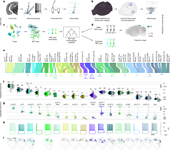
MainThe wildly varying neuronal shapes originally observed with the Golgi stain provided the first clues about the cellular complexity of the brain8,9. Our understanding of cell types has expanded greatly since then and continues to grow exponentially with recent technological advances in anatomical tracing, single-cell transcriptomic characterization and electron microscopy1,10,11,12. These techniques have revealed the cellular landscape of the brain at extraordinary scale and detail. However, in many cases, individual cellular properties have been studied in isolation, and we lack knowledge of the correspondences among them that would establish robust, integrated cell-type definitions. As cell types are the fundamental components of the brain, establishing a multimodal cell-type definition that includes morphological, molecular, connectional and functional properties will form a stable foundation for understanding brain organization and function13,14,15.Patch-seq is a powerful method that enables collection of electrophysiological, morphological and transcriptomic data from the same cell2,3. By mapping transcriptomic signatures of Patch-seq cells to an established taxonomy of transcriptomic (T) types16, we can annotate and refine these cell-type taxonomies with additional electrophysiological and morphological properties4,5,6,17. In the mouse and human neocortex, Patch-seq studies revealed that the morphoelectric properties of neurons largely supported transcriptomically identified cell types in both species, although large phenotypic variation was observed within certain T-types4,5,7. Patch-seq also led to the identification of 28 GABAergic morphoelectric–transcriptomic (MET) types, each with distinct axonal laminar innervation patterns and putative synaptic circuits4.Transcriptomic studies of cortical long-range projecting neurons have relied on RNA sequencing of retrogradely labelled neurons to assign projection target subclass identity (for example, layer 5 intratelencephalic (L5 IT)) to T-types16,18. However, the relationship between T-types and the complete long-range axonal projections of individual neurons has largely been missing from transcriptomic studies. This is a major gap in our knowledge as transcriptomic characterization of excitatory cortical neurons revealed additional cortical cell types (approximately 30 types) relative to more traditional morphoelectric characterization studies (9–19 types)16,19,20,21. Understanding the relationship between T-types and axonal projection patterns in mammals could help to explain the wider transcriptomic diversity if specific projection target properties are encoded in the transcriptomes of adult mice as they are in fruit flies22,23. Few studies describe the complete axonal projections of single neurons11,24,25,26,27,28. Furthermore, detailed axonal projection patterns of individual T-types have only been established for a small number of cell types in the mouse cortex29,30. This relationship remains unexplored for the thousands of T-types that have now been described across the whole mouse brain1 and in other mammalian species31.To address these questions here, we developed morphology-based computational approaches for cross-modality and cross-dataset integration. Focusing on excitatory neurons in the mouse visual cortex (VIS), we generated a Patch-seq dataset from which we defined 17 MET-types. Using the local morphologies of transcriptomically characterized MET-types, we established the correspondences between the multimodal profiles of Patch-seq neurons and the complete morphologies and interareal projections of a whole-neuron morphology (WNM) dataset. With this framework, we characterized integrated MET-types, examined how transcriptomic variation corresponds to electrophysiological and morphological variation within a MET-type, and built models to predict specific projection targets for individual neurons based on all these characteristics. With this approach, we provide an integrated view of transcriptomically defined excitatory neuron types and their phenotypic properties, including interareal projection patterns.Integrated taxonomy of MET excitatory neuron typesWe used Patch-seq to investigate the correspondences between transcriptomic identity and intrinsic electrophysiological and local morphological properties of excitatory neurons in the adult mouse VIS (Fig. 1a). Transgenic mice with labelling of different populations of excitatory cortical neurons were used for Patch-seq recordings (Supplementary Tables 1 and 2). In acute brain slices containing the VIS, we collected electrical responses to a standardized set of hyperpolarizing and depolarizing current stimuli, extracted the nucleus and cytosol for single-cell RNA sequencing, and filled neurons with biocytin for later morphological reconstruction. Patch-seq recordings of excitatory neurons (n = 1,528) were included in this study (75 L2/3 neurons have been previously published7 and were reanalysed as part of this study). Finally, we generated an image-based dendritic reconstruction for 689 of these neurons with adequate biocytin fills4.Fig. 1: Patch-seq and WNM data generation and integration to establish integrated MET-types.a, Schematic of the Patch-seq experimental strategy. b, Schematic of the parallel WNM experimental strategy. Integration of the two datasets is based on shared dendritic properties. c, UMAP (left) based on gene expression of dissociated cells in the reference transcriptomic taxonomy (colours indicate T-type as given in panel e), second from left: schematic of MET-type classification for cells from Patch-seq recordings, schematized morphologies for Patch-seq cells assigned to different MET-types (second from right) and MET-type morphological classifier (right) that ingests morphological features from both datasets. d, MET-types are predicted for WNM cells with known projection targets by way of the MET-type morphological classifier. SC, superior colliculus; TH, thalamus. e, River plot showing the relationships between T-types (top) and assigned MET-types (bottom) for cells from Patch-seq recordings with all three data modalities available. f, Soma distributions for Patch-seq MET-types (left side of the violin) and WNM (right side of the violin). The n is shown by MET-type for each dataset. Scale bar, 200 µm. g, Example cortical layer-aligned morphological reconstructions of dendrites. Scale bar, 200 µm. h, Example electrophysiological responses for each MET-type. Electrophysiology examples include responses evoked by a hyperpolarizing current step (−70 pA or −90 pA), and the response evoked by a rheobase +30 pA or +40 pA stimulus. Scale bar, 500 ms. i, Example WNMs registered to the Allen CCFv3 for each MET-type. Each panel shows an individual WNM located in VISp (left) and/or HVAs (right).Source dataWe collected a WNM dataset and compared it with the Patch-seq dataset to understand how local and long-range axonal phenotypes correspond to cell types defined by MET properties (Fig. 1b). We used a related set of transgenic mouse lines for WNM and Patch-seq experiments (Extended Data Fig. 1 and Supplementary Table 2). To achieve sparse labelling for the WNM dataset, the recombinase driver lines were combined with transgenic reporter lines or viral reporters. The brains were imaged using whole-brain fluorescence micro-optical sectioning tomography (fMOST)32. From these images, the complete dendritic and axonal morphology of 341 neurons was reconstructed (Fig. 1b). Images and reconstructions were registered to the Allen Common Coordinate Framework (CCFv3), and the complete set of projection targets was calculated for each neuron.Patch-seq neurons were each assigned a T-type using a reference taxonomy16 based on dissociated neurons from the primary VIS (VISp; Fig. 1c). Intrinsic electrophysiological properties and dendritic morphological features of these same neurons were analysed with respect to T-type assignments to establish 17 MET-types based on a dataset of 389 cells for which we had all three data modalities4 (Methods; Extended Data Fig. 1e). These MET-types were identified by applying a community detection algorithm to a graph where nodes represented neurons with transcriptomic and electrophysiological data and a manually curated dendritic reconstruction alongside nodes representing T-type–ME-type combinations; neuron nodes in the graph were connected to T-type–ME-type combination nodes by edges weighted by mapping probabilities and connected to each other by edges weighted by average multimodal correlations (Methods; Extended Data Fig. 1f). The community detection was run with multiple random seeds and correlation thresholds (Methods), and MET-types were assigned to 384 triple-modality cells by consensus based on co-clustering rates across runs (five cells did not reliably co-cluster with other cells and were consequently not assigned a MET-type). We also mapped our Patch-seq neurons to a recently published whole-brain transcriptomic taxonomy1 and observed a similar consolidation of those T-types into MET-types (Extended Data Fig. 3a). Given the tight links between MET-types and T-types, we used T-type labels to infer MET-type labels for an additional 1,053 cells that had electrophysiological and transcriptomic data but no manually curated morphological reconstruction (Methods).To test our ability to predict MET-types from local morphology alone, we trained a random forest classifier solely with the dendritic and soma features of MET-types. Application of this classifier to the data excluded from training showed that MET-types could be predicted with more than 90% accuracy (Extended Data Fig. 2). Therefore, the local morphology is a defining feature of most VIS MET-types and can be used to predict the MET-type for morphologically characterized neurons in this brain region.To link MET-types to neurons in the VIS WNM dataset generated as part of this study, we established a MET-type morphological classifier using dendritic morphology and projection subclass (derived transcriptomically for Patch-seq and anatomically for WNM) to generate robust, cross-platform MET-type predictions (Fig. 1c and Extended Data Fig. 2). For this analysis, the same set of dendritic features was calculated from morphological reconstructions from both datasets (Fig. 1c,d). This computational framework established an integrated taxonomy (Fig. 1e–i), enabling further interrogation of the relationships among T-type, MET-type, anatomical location, dendritic and axonal morphology, electrophysiology, transcriptomic properties and the complete interareal projection map of excitatory visual cortical neurons.MET-types were named by their laminar locations (for example, L2/3), transcriptomically derived projection types (for example, IT) and marker genes that distinguished them from other related MET-types, if present (Methods; Extended Data Fig. 3b). MET-types with the same layer and projection type were also distinguished with numerical suffixes. We note that in this study, we use the ‘IT’ label primarily to refer to the transcriptomically defined subclasses associated with those projection patterns as defined in single-cell transcriptomic taxonomies1,16,33. Other neurons, such as those in the L5 near projecting (NP) and L6b subclasses, also exhibit IT projection patterns, but as they are transcriptomically and developmentally more related to L6 corticothalamic (CT) and L5 extratelencephalic (ET) neurons1,16,34, here we present them alongside those related types.MET-types across both datasets were found predominantly in a specific layer or in two neighbouring layers, in accordance with related cell types identified in previous studies5,16,19,21,33 (Fig. 1f). When we examined the spatial distribution of MET-types across VIS (Extended Data Fig. 4), it was consistent with our sampling distribution, except for L5/L6 IT Car3. This MET-type was more frequently found in the lateral VISp and lateral higher visual areas (HVAs) such as the lateral VIS (VISl; Extended Data Fig. 4), consistent with previous studies28,33.Some MET-types probably corresponded to morphological or electrophysiological types from previous studies19,20, such as L2/3 IT, which contained wide branching neurons located throughout the depth of L2/3 (ref. 35), and L4 IT with little-to-no apical tuft and regular firing of action potentials36 (Fig. 1g,h). Both types had long-range axons mostly in nearby cortical regions, similar to previously studies in this and other brain regions11,25,28 (Fig. 1i).Other MET-types displayed dendritic or axonal profiles not previously described. L5 IT-2 had sparse tufted apical dendrites with elaborate local axon, differing from the more typical slender-tufted IT neurons found in L5 (refs. 19,35,37,38,39). The L4/L5 IT-type neurons, which were largely found in L5, had slender-tufted dendrites along with more extensive long-range axonal projections than other IT-types. Another layer-straddling IT-type, L5/L6 IT Car3, also had relatively extensive long-range projections28. This MET-type was composed of a single T-type and exhibited a stellate dendritic morphology that was particularly unusual for deep excitatory neurons. The L5 ET-1 Chrna6 MET-type also contained neurons from a single T-type with distinct gene expression compared with other thick-tufted L5 ET neurons16. The Chrna6 cells were restricted to the L5 side of the L4/L5 border, and their long-range projections were more limited than other ET-types. Overall, WNM-predicted MET-types had distinct interareal projection patterns. This morphology-based, cross-dataset mapping provides a unified, multimodal description of neuronal cell types for this brain region.Integrated MET-typesWe used morphoelectric properties of Patch-seq neurons to form a bridge from transcriptomic cell types to the previous literature and to establish robust cell-type definitions (MET-types) where multimodal properties consistently aligned. The characterization of MET-types also yielded a triple-modality ‘Rosetta stone’, potentially enabling the mapping of cells across datasets and species using a shared modality. To provide an overview of the transcriptomic, electrophysiological and morphological landscapes of Patch-seq neurons, we showed uniform manifold approximation and projection (UMAP) embeddings for each Patch-seq data modality (n = 1,528 cells with transcriptomics and electrophysiology; n = 389 of those cells that also had a manually curated morphological reconstruction; Figs. 2a–c and 3a–c). Transcriptomic UMAPs were derived from principal component analysis using 1,398 differentially expressed genes, electrophysiological UMAPs from 62 sparse principal components, and morphological UMAPs from 50 morphological features (Methods).Fig. 2: Integrated IT MET-types.a–c, UMAPs based on gene expression (a; transcriptomics (T)), electrophysiology (E; b) and morphology (M; c) from Patch-seq experiments (the colour indicates IT T-type; other T-types are in grey). d, River plot of IT T-type and MET-type correspondence. e, Example Patch-seq MET-type morphologies (left) and average dendritic depth profiles (right). f, Average action potential waveforms. The dotted line indicates the action potential waveform averaged across all cells. g, Average firing frequency versus stimulus intensity (n = 105 L2/3 IT cells, 100 L4 IT cells, 146 L4/L5 IT cells, 61 L5 IT-1 cells, 16 L5 IT-2 cells, 12 L5 IT-3 cells, 29 L6 IT-1 cells, 53 L6 IT-2 cells, 10 L6 IT-3 cells and 24 L5/L6 IT Car3 cells). Data are presented as mean ± s.e.m. Colours are as in panel f. h, Example responses to subthreshold (thick) and suprathreshold (thin) depolarizing current steps. The rise time is calculated over the interval (black) between 10% and 90% of the steady-state voltage (black). The colours indicate MET-types as in panel f. i, Rise times (left) and depolarizing ‘hump’ amplitudes (right) of L6 IT MET-types (n = 29 L6 IT-1 cells, 51 L6 IT-2 cells, 9 L6 IT-3 cells and 23 L5/L6 IT Car3 cells). MET-types were compared by Kruskal–Wallis test (P = 5.529 × 10–6 for rise times; P = 0.000572 for hump amplitudes) followed by post-hoc pairwise Dunn tests adjusted for multiple comparisons (the asterisk indicates adjusted P < 0.05; rise time: adjusted P = 1.446 × 10–5 for L6 IT-1 versus L5/L6 IT Car3, adjusted P = 1.632 × 10–5 for L6 IT-2 versus L5/L6 IT Car3; hump amplitude: adjusted P = 0.00355 for L6 IT-1 versus L5/L6 IT Car3, and adjusted P = 0.000457 for L6 IT-2 versus L5/L6 IT Car3). The bars indicate the group averages. Colours are as in panel f. j, Differentially expressed ion channels between L6 IT-1 and L5/L6 IT Car3 (L6 IT-2 and L6 IT-3 are also shown). k, Apical dendrite vertical bias versus maximum apical path distance for L6 IT MET-types. l, Example WNMs of predicted IT MET-types in CCFv3. m, WNMs in panel l aligned to an average layer space. Dendrites are shown in MET-type colours (see panel f); the local axon is shown in grey. Average dendritic and local axon depth profiles are also shown with the same colour scheme. n, UMAP based on dendritic morphology and soma location from Patch-seq and WNM (black outline) studies. o, UMAP based on local axon morphology of WNMs. p, UMAP based on complete axon morphology of WNMs. The colours indicate MET-type (Patch-seq) or predicted MET-type (WNM) in panels n–p. q, Top views of VISp and HVAs showing the locations of the VISp WNM IT neurons (top) and the visuotopic altitude (bottom). The dot size reflects the number of projection targets. r, Left, binary projection target matrix ordered by predicted MET-type, then by altitude (colours are as in panel q) within type. The bars below indicate the number of targets per neuron (see Methods for target definition). Mean ± s.e.m. projection target summaries by MET-type is also shown (right). See Methods for nomenclature and abbreviations of anatomical regions in CCFv3. The full projection target matrix is shown in Supplementary Data Table 1.Source dataFig. 3: Integrated ET, NP, CT and L6b MET-types.a–c, UMAPs based on gene expression (a), electrophysiology (b) and morphology (c) from Patch-seq experiments (the colour indicates ET, NP, CT and L6b T-types; IT T-types are in grey). d, River plot of ET, NP, CT and L6b T-type and MET-type correspondences. e, Example Patch-seq morphologies (left) and average dendritic depth profiles (right). f, Average action potential waveforms. The dotted line indicates the action potential waveform averaged across all cells. g, Average firing frequency versus stimulus intensity (n = 42 L5 ET-1 Chrna6 cells, 83 L5 ET-2 cells, 311 L5 ET-3 cells, 35 L5 NP cells, 102 L6b cells, 255 L6 CT-1 cells and 53 L6 CT-2 cells). Data are presented as mean ± s.e.m. Colours are as in panel f. h, Example L5 ET responses to depolarizing current steps showing different initial activity, including bursting. i, Maximum instantaneous firing frequency versus total evoked action potentials from depolarizing current steps. j, Differentially expressed ion channels between L5 ET-1 Chrna6 and L5 ET-3 (L5 ET-2 is also shown). k, Example WNMs of predicted L5 ET, L5 NP, L6 CT and L6b MET-types in CCFv3. l, WNMs in panel k aligned to an average layer space. Dendrites are shown in MET-type colours; the local axon is shown in grey. Average dendritic and local axon depth profiles are also shown with the same colour scheme. m, UMAP based on dendritic morphology and soma location features from Patch-seq and WNM (black outline) studies. n, UMAP based on local axon morphology features of WNMs. o, UMAP based on complete axon morphology features of WNMs. The colours indicate MET-type (Patch-seq) or predicted MET-type (WNM) in panels m–o. p, Top views of VISp showing the locations of WNM L5 ET (top) and CT and L6b (middle) neurons, as well as visuotopic azimuth (bottom). The dot size reflects the number of projection targets. q, Left, binary projection target matrix ordered first by predicted MET-type, then by azimuth within type (colours are as in panel p). The bars below indicate the number of targets per neuron (see Methods for target definition). The mean ± s.e.m. projection target summaries by MET-type are also shown (right). See Methods for nomenclature and abbreviations of anatomical brain regions in CCFv3. The full projection matrix is shown in Supplementary Table 1.Source dataIT MET-typesCells collected from Patch-seq experiments that mapped to the IT group occupied distinct regions of the transcriptomic UMAP based on their T-type but also followed an intuitive cortical layer progression (Fig. 2a). L5/L6 Car3 neurons (referred to as L6 Car3 in the reference taxonomy16) were most distinct, appearing on a separate island from the other IT T-types. In the UMAP derived from the electrophysiological features of Patch-seq neurons, T-types appear biased towards different but overlapping regions of a single, large island (Fig. 2b). The UMAP derived from morphological features of Patch-seq neurons had more discrete groupings of transcriptomically coherent cells than the electrophysiology UMAP5, with L2/3 IT, L5/L6 IT Car3 and L5 IT neurons each in distinct locations (Fig. 2c).Figure 2d illustrates how closely related IT T-types (for example, L2/3 IT Rrad and L2/3 IT Agmat) were consolidated into fewer MET-types. L6 IT T-types were an exception, splitting across three L6 IT MET-types. L4 IT Rspo1 and L6 IT Car3 had nearly one-to-one correspondences with MET-types.Patch-seq IT MET-types had distinctive morphologies, with clear differences in the length, branching pattern and orientation of their apical and basal dendrites (Fig. 2e). L5 IT-2 neurons were particularly notable among IT neurons for their minimal apical tufts, and for some cells, long basal dendrites.IT MET-types also differed in their action potential and firing properties (Fig. 2f,g and Extended Data Fig. 5a). For example, the f–I curves of L2/3 IT neurons had significantly higher rheobases than other MET-types (Kruskal–Wallis test P = 8.65 × 10−47, post-hoc Dunn tests P = 0.00182 or less) apart from L5/L6 IT Car3 neurons (post-hoc Dunn P = 0.607), which also had compact dendritic fields, consistent with previous observations of L2/3 IT neurons40. IT MET-types from L2/3 to L5 showed a consistent increase in several subthreshold properties (for example, membrane time constant and hyperpolarization-induced sag) with depth in the cortex41 (Extended Data Fig. 5b), except for L5 IT-3 Pld5, which had input resistance, membrane time constant and sag values closer to L6 IT MET-types.L5/L6 IT Car3 neurons were distinct from other L6 IT-types across modalities. They exhibited faster rise times during depolarizing current steps (Fig. 2h,i), and a number of these neurons also exhibited large depolarizing ‘humps’ at potentials just below the action potential firing threshold (Fig. 2h,i). The timing of this hump frequently corresponded to the timing of the first action potential at rheobase. L5/L6 IT Car3 cells expressed different ion channels compared with L6 IT-1 cells, including several Trpc channels (Trpc3, Trpc5 and Trpc6; Fig. 2j). L5/L6 IT Car3 cells did not express genes for P/Q-type calcium channels (Cacna1a), Kv3.4 channels (Kcnc4) or Kv5.1 channels (Kcnf1) unlike the L6 IT MET-types. These differentially expressed ion channels may contribute to the distinctive electrophysiological properties of the L5/L6 IT Car3 neurons. L5/L6 IT Car3 neurons could also be distinguished morphologically from other L6 IT cells by their smaller apical dendrites with a vertical bias towards the white-matter side of the soma (Fig. 2k).WNMs of predicted IT MET-typesAs mentioned above, a major question concerning transcriptomically defined cell types is to what extent they reflect their detailed, axonal projections. To understand the relationship between IT MET-types and the pattern of local and interareal axonal projections, we generated a dataset of 140 IT VIS neurons reconstructed from whole-brain fMOST images (see Fig. 1b). Neurons were labelled using transgenic mouse lines to achieve broad coverage across layers and projection neuron subclasses28 (Extended Data Fig. 1 and Supplementary Table 2). Where available, we used mouse lines that selectively labelled IT T-types (for example, Gnb4) and/or subclasses (for example, Cux2). We prioritized neuron reconstructions in L2/3 through L6b of VISp (n = 58), but an additional set of VIS neurons was also reconstructed in HVAs (n = 82: VISl n = 16, anteromedial visual area (VISam) n = 9, posteromedial visual area (VISpm) n = 7, postrhinal visual area (VISpor) n = 8, anterolateral visual area (VISal) n = 10, rostrolateral visual area (VISrl) n = 12, anterior visual area (VISa) n = 9, posterolateral visual area n = 5 and laterointermediate visual area (VISli) n = 6). A subset of these neurons (36 VISp, 3 VISa, 8 VISal, 4 VISam, 6 VISl, 2 VISli, 2 VISpm, 2 VISpor and 10 VISrl neurons) has been previously published28; here we re-registered these cells to CCFv3 and reanalysed them (Methods).To link MET-types defined with Patch-seq to WNM data, we used a classifier that relied on dendritic features and projection subclass assignments from both datasets (Extended Data Fig. 2). Several processing steps were performed on the WNM data to ensure feature alignment with Patch-seq data before applying the classifier (Extended Data Fig. 2). The MET labels provided by the classifier enabled analysis of the correspondence between the WNMs with respect to their predicted IT MET-type (Fig. 2l–r and Extended Data Fig. 6a,b,e).With this approach, we identified eight of the ten Patch-seq-defined IT MET-types in the VISp WNM dataset, although L6 IT-3 was only found in VISli. Example WNMs organized by MET-type assignment are shown in Fig. 2l,m (also Supplementary Information 1). The missing L5 IT-1 MET-type was probably the consequence of the small number of WNMs sampled from the L5 IT subclass, whereas the L5 IT-3 Pld5 type was excluded from the classifier because it did not meet the threshold of n > 3 Patch-seq neurons. Visually, MET-types from Patch-seq and WNM datasets, had consistent dendritic phenotypes (Fig. 2e,m and Extended Data Fig. 7). A UMAP derived from dendritic features also indicated good alignment between the two datasets (Fig. 2n and Extended Data Fig. 8a), as neurons that mapped to the same MET-type grouped together regardless of dataset. Our VISp mapping results also agreed with the T-type or subclass-specific transgenic mice from which these neurons were sampled (Extended Data Fig. 8b). For example, all predicted L5/L6 IT Car3 neurons in VISp were labelled by the Gnb4 mouse line (Extended Data Fig. 1), which labels neurons in the Car3 subclass28.We next examined the local axon (defined as the axon within a 500-µm radius cylinder centred on the soma) of the WNMs and saw clear differences across types (Fig. 2m and Supplementary Information 1). Predicted L2/3 IT neurons predominantly innervated superficial L1, L2/3 and L5 and L4 IT neurons had notably dense and highly columnar local axons, predominantly in L2/3 and L4, consistent with L4 sensory cortical neurons36. Predicted L4/L5 IT neurons had radially projecting axon that elaborated in L1 and superficial L5. By contrast, predicted L5 IT-2 neurons densely innervated L2/3 and deep L5. Predicted L6 IT-1 and L6 IT-2 had axonal projections largely restricted to L6, whereas predicted L5/L6 IT Car3 neurons had sparse axons in all layers except L1.Local axon morphology, which was not used by the Patch-seq MET-type classifier, could also distinguish WNM predicted MET-types, particularly the neurons in L6 that were grouped together in the dendrite-only UMAP (Fig. 2o and Extended Data Figs. 8c and 9). We tested how well local axon alone could predict predicted MET-types in the WNM data; the classifier achieved 70% accuracy (Extended Data Fig. 8d). These findings supported our WNM MET-type assignments by demonstrating that local axonal morphologies also differed across predicted MET-types.When we examined the long-range projections of predicted IT MET-types, we found distinct axonal properties and projection target patterns (Fig. 2p–r, Extended Data Fig. 9 and Supplementary Table 3), although there was still considerable variation across individual neurons in the specific set of targets. Organizing neurons according to their visuotopic location in altitude within VISp42 (Fig. 2q) revealed systematic differences in the set of projection targets contacted by predicted MET-types. Predicted L2/3 IT MET-types sparsely targeted three HVAs on average, with rarer projections to other cortical structures such as primary somatosensory area, barrel field (Fig. 2r). They rarely projected contralaterally, in line with previous observations25 (Fig. 2r). We also observed two ‘local’ L2/3 neurons with axons restricted to VISp (Fig. 2r). L4 IT neurons have typically been considered local neurons, and we did find examples of that in our dataset. However, most predicted L4 IT neurons projected outside VISp16,43, contacting 1–2 HVAs (Fig. 2r and Extended Data Fig. 6b). Like L2/3 ITs, predicted L4 IT neurons rarely projected contralaterally; when they did, they exclusively contacted VISp (Fig. 2r). These two superficial VISp MET-types had surprisingly similar axonal phenotypes.By contrast, predicted L4/L5 IT MET-types projected broadly across ipsilateral telencephalon and contralateral VIS, targeting 9.33 structures on average (Extended Data Fig. 9 and Supplementary Table 4), including multiple HVAs, association areas such as the anterior cingulate area and caudoputamen, and other sensory-motor areas such as secondary motor area (Extended Data Fig. 10). Over 50% of predicted L4/L5 IT neurons projected contralaterally, most consistently targeting VISp (Fig. 2r and Extended Data Fig. 10a–c). Of the three L5 IT MET-types described with Patch-seq, we only identified L5 IT-2 neurons in the WNM dataset. These neurons had extensive local projections and mainly targeted ipsilateral HVAs. They targeted VISl regardless of their visuotopic location. Unlike L4/L5 IT predicted MET-types, VISp L5 IT-2 neurons did not project contralaterally. There were stark differences between predicted L4/L5 IT and L5 IT-2 neurons in the proportion of contralaterally projecting neurons, and in the amount of axon in VIS relative to non-VIS regions. These types have previously been merged into a single, slender-tufted L5 IT group (compare with ref. 19).We identified all three L6 IT-1 MET-types in the WNM dataset, but only one cell per type. These neurons had few targets. The L6 IT-1-predicted neuron projected contralaterally, whereas the L6 IT-2 predicted neuron did not. Unlike the other IT neurons in our WNM dataset, they predominantly innervated L6 in VISp and other cortical regions. More neurons are needed to characterize the axonal projection of these three L6 IT-types.Finally, we predicted two VISp neurons and four HVA neurons to belong to the laterally located L5/L6 IT Car3 type (Fig. 2r and Extended Data Fig. 6a,b); VISp neurons projected to ipsilateral and contralateral VISp and VISl and contralateral VISrl and VISal (Fig. 2r). These neurons had stronger contralateral than ipsilateral projections based on total axon length and number of targets (Fig. 2r and Extended Data Figs. 6a,b and 10d,e).To examine the distribution of ipsilateral versus contralateral axons for all VISp-predicted IT-types, we calculated the proportion of axons that innervated VISp versus other structures. For the majority of IT MET-types, L2/3, L4, L5 IT-2 and L6 IT-1-3 (and L6b, discussed more later), the bulk of their axons remained in the ipsilateral VISp (80–90%; Supplementary Table 4). By contrast, the predicted VISp L4/L5 IT and L5/L6 IT Car3 types had the opposite pattern; more than 50% of their axon projected outside the ipsilateral VISp (notably to the contralateral cortex). However, these two types had different patterns of regions and lamina targeted in the contralateral cortex (Fig. 2r and Extended Data Figs. 6 and 10b,f,g): predicted L4/L5 IT neurons strongly innervated L1 and the border region of L4 and L5, whereas predicted L5/L6 IT Car3 neurons more strongly innervated L2/3 and upper L4 (Extended Data Fig. 10b,g).Predicted IT MET-types located in HVAs all displayed similar projection patterns to their VISp counterparts; however, there was an inverse relationship between the amount of local axon and the number of projection targets across the VISp and HVAs (Extended Data Fig. 6e). Neurons in HVAs had relatively less local axon and more axon in target regions than VISp neurons, in alignment with previous studies11. This pattern probably also has important functional implications for local versus interareal information processing across the cortex.ET, NP, CT and L6b MET-typesAs with neurons in the IT subclasses, cells collected from Patch-seq experiments that mapped to the ET, NP, CT and L6b subclasses occupied distinct locations within the transcriptomic UMAP; the L5 ET Chrna6 MET-type formed its own separate island (Fig. 3a). In the electrophysiology-based UMAP, L6b neurons were found among the region of the UMAP occupied mostly by IT neurons, whereas L5 NPs were located on a separate island (Fig. 3b), indicating distinctive electrophysiological properties for this late-developing T-type34. The UMAP derived from morphological features (Fig. 3c) showed similar relationships between the subclasses as other modalities. As with the IT subclasses, related T-types were merged into MET-types, apart from L5 ET-1 Chrna6, which was composed of a single T-type (Fig. 3d).Neurons had distinct morphologies across the L5 ET, L5 NP, L6 CT and L6b subclasses, with apical dendrites that ranged from thick tufted (L5 ET) to narrow, short and untufted (L6 CT). L5 NP neurons had particularly sparse oblique apical dendrites (Fig. 3e). These MET-types generally exhibited similar action potential waveforms, with the L5 ET MET-types having somewhat narrower and L6b having somewhat broader action potentials (Fig. 3f and Extended Data Fig. 5d). Cells in the L5 NP MET-type were more excitable with a significantly lower rheobase than the other MET-types (Fig. 3g and Extended Data Fig. 5d; Kruskal–Wallis P = 5.39 × 10−56, post-hoc Dunn P ≤ 0.00158 for L5 NP versus other types). L5 NP neurons also had a higher input resistance (Kruskal–Wallis P = 1.22 × 10−92, post-hoc Dunn P ≤ 3.35 × 10−4) and longer membrane time constant (Kruskal–Wallis P = 3.65 × 10−25, post-hoc Dunn P ≤ 0.000281) than the other MET-types (Extended Data Fig. 5e,f), whereas L5 ETs had lower average input resistances. All these MET-types exhibited hyperpolarization-induced sag, but it was significantly less pronounced in L6b neurons than in the others (Extended Data Fig. 5e,f; Kruskal–Wallis P = 3.18 × 10−74, post-hoc Dunn P ≤ 7.59 × 10−11). L6 CT-1 neurons could be distinguished from L6 CT-2 neurons by their lower resting potentials (post-hoc Dunn P = 0.0116) and input resistances (post-hoc Dunn P = 7.38 × 10−5) and correspondingly higher rheobase (post-hoc Dunn P = 1.14 × 10−12; Fig. 3g and Extended Data Fig. 5d,e).The L5 ET-1 Chrna6 cells, along with L5 ET-2 cells, typically did not fireaction potential bursts during depolarizing current steps, unlike many of the L5 ET-3 cells (Fig. 3h). This could be seen by comparing the maximum instantaneous firing frequency during a current step to the total number of action potentials fired during that step (Fig. 3i): cells that fired bursts had very high instantaneous frequencies but only fired a few action potentials. In addition, several voltage-gated ion channels were differentially expressed between L5 ET-1 Chrna6 and L5 ET-3 (Fig. 3j), including a T-type calcium channel (Cacna1h) that was expressed in L5 ET-3 but not in L5 ET-1 Chrna6 cells.WNMs of predicted ET, NP, CT and L6b MET-typesTo understand the local and interareal axonal projections of the EP, NP, CT and L6b MET-types, we generated a dataset of 202 VIS cortical neurons reconstructed from whole-brain fMOST images (Figs. 1b and 3k–q). As with IT neurons, we used transgenic mouse lines and viral strategies to capture all projection neuron subclasses (Extended Data Fig. 1 and Supplementary Table 2), as well as lines that selectively labelled T-types (that is, Chrna6-IRES2-FlpO-WPRE-neo) and/or subclasses (that is, Nxph4-T2A-CreERT2; Nxph4 is a marker gene for L6b subclass neurons).We identified all L5 ET, L5 NP, L6 CT and L6b MET-types in the WNM dataset (Fig. 3k–q). Of note, although the transgenic line labelling a neuron was not used as part of our classification, we still found that 11 out of 14 neurons reconstructed in the T-type-specific Chrna6-IRES2-FlpO mice mapped to the L5 ET-1 Chrna6 MET-type (for comparison, in the Patch-seq dataset, 22 out of 24 neurons from the Chrna6-IRES2-FlpO mice mapped to the L5 ET VISp Chrna6 T-type; Extended Data Fig. 1). The remaining three WNMs mapped to L5 ET-2 (2) and L4 IT (1). This finding served to validate our MET-type predictions for these neurons. At the subclass level, all L6b-assigned neurons were labelled by the L6b-selective Nxph4-CreER line. When we compared MET-types across datasets, we found consistent dendritic phenotypes (Fig. 3e,l,m and Extended Data Fig. 11).The local axon of these predicted MET-types also exhibited clear differences across types (Fig. 3l,n and Extended Data Fig. 8). Predicted L5 ET neurons had relatively little local axon, which was distributed in L5 and, to varying degrees, in L1 (with L5 ET-2 having the most L1 axon). Predicted L5 NP neurons had abundant local axon in L6. Predicted L6 CT neurons had wedge-shaped or very narrow local axons restricted to L4–L6. Deeper predicted L6 CT neurons also possessed one or two axon collaterals that reached L1. Predicted L6b neurons most strongly innervated L1, which agrees with previous descriptions of these neurons44.Predicted L5 ET neurons had many interareal projection targets in common, regardless of MET-type, including multiple thalamic, tectal and pretectal nuclei (Fig. 3q and Supplementary Table 3). However, predicted L5 ET-1 Chrna6 neurons had significantly fewer projection targets per neuron on average than predicted L5 ET-2. This was largely the result of fewer cortical targets (Extended Data Fig. 6 and Supplementary Table 4; Kruskal–Wallis P = 3.54 × 10−8, post-hoc Dunn P = 1.25 × 10−2). The Chrna6 cell type emerges later in development than other ET-types, which may contribute to the observed differences in axonal projection patterns34. Of the L5 ETs, predicted L5 ET-2 neurons tended to have a higher proportion of hypothalamus-targeting, caudoputamen-targeting and pons-targeting neurons (Fig. 3q; for hypothalamus, Benjamini–Hochberg false discovery rate adjusted P = 5.85 × 10−3, Supplementary Table 4). These neurons were more frequently located in the part of the VISp representing higher azimuth visual space (Fig. 3p,q). Predicted L5 ET-3 neurons had the largest apical dendrites and more reliably targeted thalamic structures than predicted L5 ET-2 (Fig. 3q and Extended Data Fig. 11).The few predicted L5 NP neurons identified in the WNM dataset were found only in HVAs (probably due to sampling). This is a relatively recently described cortical cell type45. In our study, predicted L5 NP neurons contacted the VISp and 2–5 other VIS regions, which was a relatively small number of targets for L5 HVA neurons. To our knowledge, this is the first description of the axonal targets of individual NP neurons. We note that these neurons are transcriptomically most closely related to CT neurons. However, they emerge during development at the same time as L2/3 and L4 IT neurons (embryonic day 18.5)34 and their axonal morphologies and projection patterns are similar to these superficial IT-types.The L6 CT-1-predicted and CT-2-predicted MET-types had significantly fewer targets than all L5 ET-types (Supplementary Table 4, Kruskal–Wallis P = 8.49 × 10−13, post-hoc Dunn P ≤ 8.16 × 10−4). Within the cortex, they rarely projected outside of the VISp. In the thalamus, they most reliably targeted the dorsal part of the lateral geniculate complex (LGd)-core, LGd-shell and other thalamic nuclei (Extended Data Fig. 3q). The predicted L6 CT-2 neurons tended to target the lateral posterior nucleus of the thalamus (LP) more frequently than the predicted L6 CT-1 neurons.L6b neurons, which are derived from subplate neurons, are the early pioneers of cortical development. Predicted L6b neurons most consistently targeted ipsilateral HVAs, anterior cingulate area, dorsal part/ventral part and retrosplenial area, lateral agranular part (Fig. 3q and Extended Data Fig. 6c–e). VISp-predicted L6b neurons had significantly more local axon than predicted L6b neurons in HVAs (Supplementary Table 4, Mann–Whitney Benjamini–Hochberg false discovery rate adjusted P = 4.87 × 10−3), although they had similar total axon lengths. We also found that predicted L6b neurons, regardless of soma region, consistently innervated cortical L1 (Supplementary Information 1). There were no significant differences in the number of targets for the VISp-predicted and HVA-predicted L6b neurons. This contrasts with later-developing IT-projecting neurons, where the number of projection targets increased for HVA neurons compared with VISp neurons (Extended Data Fig. 6e).Transcriptomic variation and cross-modal correspondenceAlthough our MET-type classification procedure often merged several T-types into a single MET-type, it was not the case that all neurons within a MET-type had homogeneous electrophysiological and morphological features. Indeed, we observed that neurons even within a specific T-type could exhibit a range of properties. We therefore investigated whether these variations were coordinated across modalities. To do so, we performed sparse reduced-rank regression (RRR)14 to determine how well a subset of highly variable genes in a transcriptomic subclass could predict the electrophysiological and morphological properties of those cells. In this method, a set of weights is identified for a sparse set of genes to calculate a small number of latent factors; a second set of weights is determined that produce the best prediction of the electrophysiological and morphological features (Fig. 4a). The procedure was applied separately for electrophysiological and morphological features, with different latent factors calculated for each modality. The optimal number of latent factors (the rank) and sparseness penalty hyperparameters were determined for each subclass and modality by cross-validation (Methods; Extended Data Fig. 12a–c); in addition, 15% of cells were held out to form a test dataset.Fig. 4: Sparse RRR analysis of multimodal Patch-seq data.a, Schematic illustrating sparse RRR analysis for electrophysiology (top) and morphology (bottom). A weighted subset of genes was used to calculate a small number of latent factors, which were then used to predict electrophysiological or morphological features. Electrophysiological and morphological regressions were calculated independently from each other and for each transcriptomic subclass. b–g, Bi-plots of the first two latent factors (or sole latent factor if rank = 1) for L2/3 IT (b), L4 and L5 IT (c), L6 IT (d), L5 ET (e), L6 CT (f) and L6b (g) cells. Latent factors were calculated from genes (left) and features (right) for electrophysiology (top) and morphology (bottom). Genes and features having the highest correlations with latent factors are shown; the dotted circle indicates a correlation equal to 1. The colour indicates MET-type, and the black borders indicate held-out cells not used to fit the regressions (15% of each set). EMD, earth mover’s distance; pct., percentage; std., standard deviation. h, R2 values for prediction of electrophysiology (blue) and morphology (orange) across subclasses. The darker shades indicate average cross-validated R2 (CV), and the lighter shades indicate R2 values from hold-out cells. i, Mean action potential (AP) width versus first electrophysiology latent factor (E-LF-1) for L2/3 IT neurons. Latent factors in panels i–p were calculated from gene expression data. j, Average AP waveforms for L2/3 IT cells binned by E-LF-1 value. Data are presented as mean ± s.e.m. k, Correlation between E-LF-1 and VISal/VISpm projection-related eigengene. The dotted line indicates a value of 0 on the y axis. l, Input resistance versus first electrophysiology latent factor (E-LF-1) for L6b neurons. m, Average responses to hyperpolarizing current steps (–90 pA) for L6b cells binned by the E-LF-1 value. Data are presented as mean ± s.e.m. n, Maximum apical dendrite path distance versus first morphological latent factor (M-LF-1) for L6 CT neurons. o, Soma depth versus second morphological latent factor (M-LF-2) for L6 CT neurons. p, Example L6 CT morphologies ordered and coloured by M-LF-1. The dashed line indicates prediction of the sparse RRR model, and the black borders indicate held-out cells (i,l,n,o).Source dataAfter performing sparse RRR, we could observe the relationships between specific genes, specific electrophysiological and morphological features, and the latent factors by the use of bi-plots14 (Fig. 4b–g), which illustrated how MET-types within a subclass are distributed in the latent space, with latent factors estimated from both gene expression values (Fig. 4b–g, left plots) and features (Fig. 4b–g, right plots). They also illustrated individual genes and features that are highly correlated with those dimensions. The first one or two latent factors are shown in Fig. 4b–g; additional latent factors (if present) are shown in Extended Data Fig. 13. Cells that were held out of the regression fits (points with black borders) showed similar relationships as the training data, suggesting that the observed correspondences were not primarily due to overfitting.In most subclasses, the first electrophysiology-related latent factor was associated with action potential shape features (for example, width, depth of the trough and the upstroke:downstroke ratio). Morphological latent factors were frequently associated with the size and complexity of the apical dendrite, the depth of the cell in the cortex and the amount of overlap between the apical and basal dendrites. The genes that were correlated with latent factors represented a number of gene families, including cell-adhesion molecules (for example, Cdh13, Car2, Car4, Cntn4, Tpbg, Nptx2 and Cntnap4), and synaptic (Syt2, Syt17 and Rab3b), calcium-binding (Calb1) and receptor (Chrnb3 and Gpr88) proteins. Overall, the sparse RRR procedure had similar performance for electrophysiological and morphological features within a subclass; we also observed that performance on the held-out test datasets were generally similar to the cross-validated estimates (Fig. 4h). We note that the performance of sparse RRR was poor for the L5/L6 IT Car3 and L5 NP subclasses; this could be due to several factors, including potentially insufficient data (Extended Data Fig. 12c) as well as more homogeneity in features for those subclasses. Although sparse RRR was performed independently for electrophysiology and morphology, we found that, within a subclass, the latent factors identified for each modality often were correlated with each other (Extended Data Fig. 12d), suggesting that the transcriptomic gradients that correspond with phenotypic variation are shared to some extent.We also looked at whether the latent factors identified by sparse RRR were related to the overall transcriptomic variability within subclasses as characterized by transcriptomic principal components (Tx PCs) that contributed to the T-type definitions in the original taxonomy16 and distinguished T-types within subclasses (Extended Data Fig. 14a,b). Sparse RRR latent factors often were correlated with Tx PCs (Extended Data Fig. 14c,d), suggesting that the major axes of transcriptomic variation across related MET-types were aligned with phenotypic variation as well. Unlike other subclasses, the first Tx PC of L2/3 IT neurons did not have a latent factor counterpart but was highly correlated with activity-dependent gene expression (Extended Data Fig. 15a,d), consistent with the results of Tasic et al.16 who reported that activity-dependent genes were differentially expressed across the L2/3 IT T-types. Several activity-dependent genes (for example, Fos, Fosb and Npas4) exhibited increased expression in Patch-seq cells compared with the reference dissociated dataset16 (Extended Data Fig. 15e,f), which probably results in more Patch-seq cells mapping to L2/3 IT T-types associated with high-activity states46.To further illustrate the results of the sparse RRR fits, we made predictions of electrophysiological and morphological features based on the latent factors calculated from gene expression data (Methods; Fig. 4i–o). For example, variation in the action potential width of L2/3 IT neurons could be explained well by the first electrophysiology latent factor (L2/3 IT E-LF-1; Fig. 4i), with higher latent factors predicting narrower action potentials (Fig. 4j). We also found that this latent factor was associated with a projection-related gene signature of L2/3 IT neurons observed in a previous study47 (Fig. 4k).Other electrophysiological properties of certain subclasses had close relationships with specific latent factors, such as L6b E-LF-1 and input resistance (Fig. 4l,m). Certain morphological features also could be predicted well by particular latent factors; for example, the maximum path distance in the apical dendrite could be predicted well by L6 CT M-LF-1 (Fig. 4n), whereas L6 CT M-LF-2 was predictive of cortical cell depth (Fig. 4o). Colouring example morphologies by their L6 CT M-LF-1 visualized the relationship between the variation in the apical dendrite and the latent factor (Fig. 4p).Linking multimodal properties across datasetsAs described above, a morphological classifier could reliably link MET-type identity (and the corresponding MET properties) to the complete axonal phenotype of excitatory neurons (see Figs. 2 and 3). Doing this revealed distinct patterns of interareal projections across MET-types but still showed considerable variation among the sets of targets of individual neurons belonging to the same MET-type. As local dendritic and electrophysiological properties could be predicted by gene expression in the Patch-seq dataset (see Fig. 4), we hypothesized that transcriptomic variation might relate to axonal projection features as well. Because we lack direct transcriptomic data for the WNM dataset, we used the weights from the sparse RRR fits to estimate the latent factors from the local dendritic properties of each WNM neuron (Fig. 5a). The same dendritic features were measured from WNM and Patch-seq neurons, allowing latent factors to be calculated in the same way across datasets (as when producing the right side of the Patch-seq morphology bi-plots in Fig. 4). Doing this enabled us to infer the relationship between transcriptomic gradients (represented by the latent factors) and axonal properties.Fig. 5: Relating multimodal properties to axonal projection features.a, Schematic illustrating estimation of latent factors from WNM morphological features using a sparse RRR fit from the Patch-seq data. All latent factor values in this figure were calculated from morphological features (as there is no gene expression data for WNM cells) and were specific to each subclass. b, Example L2/3 IT WNM morphologies ordered and coloured by M-LF-1 (left), and loadings of the second local axon depth PC-2 (right). c, Correlation between M-LF-1 and depth PC-2 for L2/3 IT WNM neurons (Spearman r = −0.52; adjusted P = 0.000392). d, Example L4 and L5 IT WNM morphologies ordered and coloured by M-LF-2 (left), and loadings of the third axon depth profile principal component (depth PC-3; right). Dendrites are coloured by latent factor value, and axons are in grey (b,d). e, Correlation between M-LF-2 and depth PC-3 for L4 and L5 IT WNM neurons (Spearman r = −0.67; adjusted P = 2.94 × 10−8). f, Cortical flat map visualizations of example L2/3 IT WNM morphologies ordered and coloured by M-LF-1 (only visual areas are shown in these flat maps). g, Correlation between M-LF-1 and length of axon in visual areas for L2/3 IT WNMs (Spearman r = 0.60; adjusted P = 0.000027). h, Example L4 and L5 IT WNMs ordered and coloured by M-LF-1. i, Correlation between M-LF-1 and length of complete axonal arbor for L4 and L5 IT WNMs (Spearman r = 0.70; adjusted P = 2.55 × 10−9). Spearman tests were two-sided and adjusted for multiple comparisons (c,e,g,i). j, Spearman correlations between local axon features and morphological latent factors by subclass. k, Spearman correlations between complete axon features and morphological latent factors by subclass. Only statistically significant correlations after multiple test correction are shown (j,k).Source dataWe observed multiple correlations between the transcriptomic-related latent factors and local axonal properties (Fig. 5b–e,j). For example, in L2/3 IT cells, the depth profile of local axon innervation as characterized by the second principal component (depth profile PC-2) was correlated with its morphological latent factor (Fig. 5b,c); this latent factor is also correlated with features such as depth in the cortex and the overlap of apical and basal dendrites (see Fig. 4b). The depth profile PC-2 feature had higher values for axon arbors with more innervation of L1 and lower values for arbors with more innervation of L2/3. Among L4 and L5 IT cells, lower values of their M-LF-2 (correlated with fewer apical branches; see Fig. 4c) were associated with greater innervation of L2/3, as opposed to higher values that were associated with innervation of L1 and upper L5 (Fig. 5d,e). This latent factor gradient also was associated with MET-type differences: neurons with predicted L4 IT and L5 IT-2 MET-types typically had low values of M-LF-2, whereas L4/L5 IT neurons had high values (Fig. 5e).Properties of the complete axonal arbors were also correlated with the sparse RRR-derived latent factors (Fig. 5f–i,k). For L2/3 IT cells, the length of axons found in visual cortical areas was correlated with its morphological latent factor (Fig. 5f,g). The first latent factor (M-LF-1) of L4 and L5 IT cells was positively correlated with the length of the entire axonal arbor (Fig. 5h,i). Overall, many axonal arbor features were significantly correlated with various latent factors across subclasses (Fig. 5j,k), suggesting that transcriptomic differences are associated with differences in local and long-range projection patterns.Predicting projection probabilities from individual cell characteristicsGiven that transcriptomic-related latent factors are strongly related to general features of axonal arbors, we next tested whether integrated multimodal properties of individual neurons could also predict specific projection targets. We used logistic regression with the VISp WNM dataset to model the probability of projection to target brain regions based on the sparse RRR-derived latent factors and cortical surface location.First, we fit models of projection probability based on the morphological latent factors (calculated from the morphological features of WNMs) for each subclass that had sufficient data in VISp (L2/3 IT, L4 and L5 IT, L5 ET and L6 CT; see Methods for subclass and region selection criteria). We identified models that outperformed a null model by the corrected Akaike information criterion (AICc; Methods; Extended Data Fig. 16a): negative ∆AICc values indicated better performance than a null model. Models based on latent factors generally performed better for the L4 and L5 IT and L5 ET subclasses than for the L2/3 IT and L6 CT subclasses (Extended Data Fig. 16a,b).Because VISp is visuotopically organized and because HVAs differ in their representations of parts of visual space42, we next asked how well the location of a cell in VISp could predict its projection targets. Projections to cortical regions could frequently be predicted by the projected surface location in VISp, especially for the L4 and L5 IT and L5 ET subclasses; projections to the caudoputamen and pontine grey for L5 ET neurons could also be predicted by models based on location (Extended Data Fig. 16c). For cortical regions, we generally observed higher probabilities of projection for locations nearer the target region (Extended Data Fig. 16d,g): for example, cells in medial VISp were more likely to project to VISpm, whereas cells in the anterolateral VISp tended to project to the VISrl and VISl. We also tested whether models that used both latent factor and location information outperformed the null models and found multiple cases where they did (Extended Data Fig. 16e). Finally, we identified the best-performing model type for each region and estimated the explanatory power by leave-one-out cross-validation (Extended Data Fig. 16f,g).Using these models, we examined how projection probabilities varied across a range of latent factor values and VISp locations (Fig. 6). For example, among L4 and L5 IT neurons (Fig. 6a), latent factor values similar to L4 IT cells (lower left subpanel) predicted lower projection probabilities in the target regions, whereas latent factors similar to L4/L5 IT (upper right subpanel) neurons predicted higher projection probabilities; latent factors similar to L5 IT-2 neurons (lower right subpanel) produced lower projection probabilities for retrosplenial area, dorsal part and retrosplenial area, lateral agranular part than L4/L5 IT, but higher probability for caudoputamen than L4 IT.Fig. 6: Predicting target projection probabilities.a, Predicted probabilities of L4 and L5 IT neurons projecting to cortical (middle) and subcortical (right) targets for different locations in the latent factor space (left); each subpanel corresponds to a different location in the latent factor space indicated by the red markers. The latent factor values are shown for WNM (larger markers) and Patch-seq (smaller markers) neurons; latent factors here were calculated from morphological features. The colours indicate MET-type (assigned or predicted). The cortical regions are shown as a flat map projection of ipsilateral (left) and contralateral (right) hemispheres. The regions with predictions are labelled. b, Predicted probabilities of L4 and L5 IT neurons projecting to cortical targets for different locations within the VISp (red markers). The same cortical flat map projection is used as in panel a. c, Same as panel a but for L5 ET neurons, and only the ipsilateral cortical flat map is shown, along with subcortical target regions. d, Same as panel b but for L5 ET neurons. Only the ipsilateral cortical flat map is shown, along with subcortical target regions. e, Predicted projection probabilities for two example L4 and L5 IT neurons compared with actual projections of those neurons. Predictions are from models fit on all other cells in the subclass (excluding the predicted cell). The colours indicate predicted probability; a black border indicates that the example neuron did project to that region. Only subcortical regions with predicted probabilities are shown. f, Same as panel e but for two example L5 ET cells. Anatomical regions are defined in the Methods.Source dataThe predicted probability that L4 and L5 IT MET neurons project to ipsilateral cortical targets was strongly dependent on the proximity of the neuron to those regions (Fig. 6b). Locations in the centre of VISp had lower probabilities of projecting to most regions. Projection probabilities to the contralateral VISp were higher for the lateral and anterior VISp locations.For L5 ET neurons, the probability of projecting to a subcortical target was more affected by variation in latent factor values than projections to cortical targets (Fig. 6c). Subcortical regions varied in their dependencies on the different latent factors (Fig. 6c and Extended Data Fig. 16g); for example, the probability of projecting to LGd-co depended most on M-LF-2, whereas the probability of projecting to the LP varied with both M-LF-1 and M-LF-2.The predicted probability that L5 ET neurons project to cortical targets was also strongly dependent on their locations within the VISp (Fig. 6d), as with L4 and L5 IT neurons, although the probabilities were typically lower than for L4 and L5 IT neurons at the same location (Fig. 6b,d). The location also influenced several subcortical target probabilities: for example, a more anterior location predicted a higher probability of projecting to the caudoputamen and pontine grey.We also examined individual cell target predictions based on models fit on all cells in the subclass except for the predicted cell (Fig. 6e,f and Extended Data Fig. 16f). Note that we only visualized probabilities for models of regions that outperformed a null model. Although the model predictions are probabilistic, meaning that we would not expect absolute agreement between, for example, a thresholded model prediction and actual data, we generally found that regions with high prediction probabilities were often targeted by the actual neuron (and vice versa), indicating the utility of using cortical location and transcriptomically related morphological characteristics in understanding the diversity of connectivity patterns across the brain.DiscussionIn this study, we collected and integrated a large Patch-seq and WNM dataset of excitatory neurons in the mouse VIS. We used Patch-seq data to define 17 excitatory MET-types and mapped these types to the WNMs to describe MET-type axonal properties. We identified novel L5 IT and ET integrated cell-type signatures, characterized transcriptomically related phenotypic properties within and across MET-types, and discovered gene expression patterns predictive of axonal targets.Several of the 17 excitatory MET-types had one-to-one correspondences with T-types. L5/L6 IT Car3 was one of these types, and our Patch-seq experiments characterized them as deep spiny stellate neurons, similar to local L4 neurons in appearance36. However, the predicted L5/L6 IT Car3 WNMs had elaborate long-range axons, projecting extensively to the contralateral VIS. Compared with other contralaterally projecting types, such as L4/L5 IT, they had significantly more of their total axon in the contralateral cortex (Extended Data Fig. 10; Kruskal–Wallis P = 2.00 × 10−2, post-hoc Dunn P ≤ 4.65 × 10−2). L5/L6 IT Car3 and L4/L5 IT neurons also innervated different layers in the contralateral cortex, suggesting distinct roles in interhemispheric signalling. Neurons with the predicted L5 IT-2 MET-type also had a very different local laminar innervation pattern than these other L5-centric IT MET-types, predominantly innervating L2/3. More data are needed to understand the specific role of each of these types in the cortical circuit.Within the L5 ET MET-types, the L5 ET-1 Chrna6 type was distinctive across all modalities. L5 ET-1 Chrna6 neurons rarely fired bursts of action potentials, unlike most of the L5 ET-3 cells (but like L5 ET-2 cells). Similarly, Chrna6 neurons had many fewer targets than other L5 ET-types, targeting the VIS or brainstem regions less frequently than L5 ET-2 and ET-3, respectively. Given these differences, L5 ET-types may serve distinct functional roles in the VIS, as they do in the motor cortex29.From our Patch-seq experiments, we found that transcriptomic variation (as quantified by sparse RRR latent factors) often was predictive of electrophysiological and morphological feature variation; however, this did not necessarily translate into strict separability between T-types along these feature dimensions, as T-types can be distributed within transcriptomic space in complex ways (Extended Data Fig. 14a). Still, characterizing the relationships between transcriptomics, electrophysiology and morphology allows us to understand how multimodal properties interrelate in MET-types and T-types.Using logistic regression models to predict specific projection targets from multimodal cell properties, we found that the location of the projecting cell within the VISp was important for many target regions (for example, HVAs and the caudoputamen), whereas latent factors were important for others (for example, the LP and LGd). The subclass-specific morphological latent factors create a useful link between the transcriptomic taxonomy and dendritic properties, narrowing the transcriptomic space for cross-dataset morphological mapping. In addition, neurons on one end of certain dendritic continua can display preferential targeting compared to the other end (Figs. 5 and 6), suggesting that there could be genes that encode and/or give access to MET-types that project to specific brain regions. Highly weighted genes from sparse reduced-rank regression fits (Fig. 4 and Extended Data Fig. 13) could be potential candidates for this: for example, LP-targeting L5 ET cells might be selected by identifying cells of thaT-type with high Rxfp1 expression. These analyses thus allow us to go beyond transcriptomic descriptions of major projection subclasses (for example, ET, IT and CT) by characterizing other factors that link them to specific projection targets.In the future, larger WNM datasets built from cell type-specific and subclass-specific viral and transgenic tools will help to validate our integrated cell types and address the remaining variance in axonal targeting pattern observed within types48,49. The excitatory VIS MET-type taxonomy and computational framework for cross-dataset, cross-modality mapping described can also enable integration with other important data modalities, such as synaptic connectivity4,50. Comprehensive, multidimensional descriptions of cell types and circuits that include gene expression patterns will provide an essential foundation to accelerate our understanding of the brain.MethodsAnimal care and useExperimental procedures that involved the use of mice were all conducted with approved protocols in accordance with NIH (US National Institutes of Health) guidelines. They were also approved by the Allen Institute for Brain Science Institutional Animal Care and Use Committee.Mice were housed with five or less mice per cage and were maintained on a 12-h light–dark cycle, in a humidity-controlled and temperature-controlled room with water and food available ad libitum.Transgenic mice and sparse labellingTransgenic driver and reporter mice used in Patch-seq and WNM studies are listed in Supplementary Table 1 (Patch-seq only) and Supplementary Table 2. Characterization of the expression pattern of many of the transgenic mouse lines can be found in the AIBS Transgenic Characterization database (http://connectivity.brain-map.org/transgenic/search/basic)51. Many of the brains used for WNM studies were described in a previous article28. Additional brains were sparsely and robustly labelled for WNMs studies using Supernova virus, which was provided as a gift by M. Luo as pAAV-TRE-fDIO-GFP-IRES-tTA (Addgene plasmid #118026; http://n2t.net/addgene:118026; RRID: Addgene 118026), and variants.Tissue processing and slicing procedureFor preparation of acute brain slices, adult male and female mice (postnatal day 45 (P45)–P70 of age) were first fully anaesthetized by 5% isoflurane inhalation. Intracardiac perfusion was then performed with 25–50 ml of ice-cold cutting artificial cerebrospinal fluid (ACSF; 0.5 mM calcium chloride (dehydrate), 25 mM d-glucose, 20 mM HEPES buffer, 10 mM magnesium sulfate, 1.25 mM sodium phosphate monobasic monohydrate, 3 mM myo-inositol, 12 mM N-acetyl-l-cysteine, 96 mM N-methyl-d-glucamine chloride, 2.5 mM potassium chloride, 25 mM sodium bicarbonate, 5 mM sodium l-ascorbate, 3 mM sodium pyruvate, 0.01 mM taurine and 2 mM thiourea (pH 7.3), which had been continuously bubbling with a mixture of 95% O2–5% CO2). Sections (350 µm) were sliced on a vibrating microtome (Compresstome VF-300 vibrating microtome, Precisionary Instruments or VT1200S Vibratome, Leica Biosystems), either coronally or at a 17° angle from the coronal plane. For the VIS, this latter slice angle helps to maximize the integrity of neuronal processes. To optimize registration to the CCFv3, a block-face image was collected before each section was cut (Mako G125B PoE camera with custom integrated software). Immediately after slicing, brain slices were placed in warm (34 °C) oxygenated cutting ACSF for 10 min, then allowed to further recover in holding ACSF (2 mM calcium chloride (dehydrate), 25 mM d-glucose, 20 mM HEPES buffer, 2 mM magnesium sulfate, 1.25 mM sodium phosphate monobasic monohydrate, 3 mM myo-inositol, 12.3 mM N-acetyl-l-cysteine, 84 mM sodium chloride, 2.5 mM potassium chloride, 25 mM sodium bicarbonate, 5 mM sodium l-ascorbate, 3 mM sodium pyruvate, 0.01 mM taurine and 2 mM thiourea (pH 7.3)), bubbling with a mixture of 95% O2–5% CO2 at room temperature until transferred to the microscope for recordings.Patch-clamp recordingSlices were bathed in warm (34 °C) recording ACSF (2 mM calcium chloride (dehydrate), 12.5 mM d-glucose, 1 mM magnesium sulfate, 1.25 mM sodium phosphate monobasic monohydrate, 2.5 mM potassium chloride, 26 mM sodium bicarbonate and 126 mM sodium chloride (pH 7.3) and continuously bubbled with 95% O2–5% CO2. The bath solution contained blockers of fast glutamatergic (1 mM kynurenic acid) and GABAergic synaptic transmission (0.1 mM picrotoxin). Thick-walled borosilicate glass (G150F-3, Warner Instruments) electrodes were manufactured (Narishige PC-10) with a resistance of 4–5 MΩ. Before recording, the electrodes were filled with approximately 1.0–1.5 µl of internal solution with biocytin (110 mM potassium gluconate, 10.0 mM HEPES, 0.2 mM ethylene glycol-bis (2-aminoethylether)-N,N,N′,N′-tetraacetic acid, 4 mM potassium chloride, 0.3 mM guanosine 5′-triphosphate sodium salt hydrate, 10 mM phosphocreatine disodium salt hydrate, 1 mM adenosine 5′-triphosphate magnesium salt, 20 µg ml−1 glycogen, 0.5 U µl−1 RNAse inhibitor (2313A, Takara) and 0.5% biocytin (B4261, Sigma), pH 7.3). The pipette was mounted on a Multiclamp 700B amplifier headstage (Molecular Devices) fixed to a micromanipulator (PatchStar, Scientifica).Electrophysiology signals were recorded using an ITC-18 Data Acquisition Interface (HEKA). Commands were generated, signals processed and amplifier metadata were acquired using MIES (https://github.com/AllenInstitute/MIES/), written in Igor Pro (Wavemetrics). Data were filtered (Bessel) at 10 kHz and digitized at 50 kHz. Data were reported uncorrected for the measured liquid junction potential of −14 mV between the electrode and bath solutions. Before data collection, all surfaces, equipment and materials were thoroughly cleaned in the following manner: a wipe down with DNA away (Thermo Scientific), RNAse Zap (Sigma-Aldrich) and finally with nuclease-free water.After formation of a stable seal and break-in, the resting membrane potential of the neuron was recorded (typically within the first minute). A bias current was injected, either manually or automatically using algorithms within the MIES data acquisition package, for the remainder of the experiment to maintain that initial resting membrane potential. Bias currents remained stable for a minimum of 1 s before each stimulus current injection.To be included in the analysis, neurons needed to have a more than 1 GΩ seal recorded before break-in and an initial access resistance of less than 20 MΩ and less than 15% of the cell Rinput. To stay below this access resistance cut-off, cells with a low input resistance were targeted with larger electrodes. For an individual sweep to be included for analysis, the following criteria were applied: (1) the bridge balance was less than 20 MΩ and less than 15% of Rinput; (2) bias (leak) current within ±100 pA; and (3) root mean square noise measurements in a short window (1.5 ms, to gauge high-frequency noise) and longer window (500 ms, to measure patch instability) of less than 0.07 mV and less than 0.5 mV, respectively.After electrophysiological recording, the pipette was centred on the soma or placed near the nucleus (if visible). A small amount of negative pressure was applied (approximately −30 mbar) to begin cytosol extraction and to attract the nucleus to the tip of pipette. After approximately 1 min, the soma visibly shrank and/or the nucleus was near the tip of the pipette. While maintaining negative pressure, the pipette was slowly retracted; slow, continuous movement was maintained while monitoring the pipette seal. Once the pipette seal reached more than 1 GΩ and the nucleus was visible on the tip of the pipette, the speed was increased to remove the pipette from the slice. The pipette containing internal solution, cytosol and the nucleus was removed from pipette holder, and its contents were expelled into a PCR tube containing the lysis buffer (634894, Takara). Metadata for all Patch-seq neurons including in this study are in Supplementary Table 1.Electrophysiology feature analysisElectrophysiological features were measured from responses elicited by short (3 ms) current pulses and long (1 s) current steps as previously described4,21. Action potentials were detected, and the threshold, peak, fast trough and width (at half-height) were calculated for each action potential along with the ratio of the peak upstroke dV/dt to the peak downstroke dV/dt (upstroke:downstroke ratio). Several voltage trajectories (the initial action potential elicited by the lowest-amplitude current pulses and steps, the derivatives of those action potentials, and the interspike interval) were analysed as previously described. Action potential features across responses to long current steps were averaged in time bins and concatenated across step amplitudes; bins without action potentials had interpolated values from their neighbours. This was done for steps starting at a given rheobase for a cell and increasing at 10-pA intervals. Sweeps from intervals without data were interpolated from sweeps at neighbouring intervals. Subthreshold responses to hyperpolarizing current steps were analysed as before by downsampling to 10-ms bins and concatenating responses from different stimulus amplitudes (ranging from −90 pA to −10 pA). Sparse principal component analysis was performed separately on data from each of these categories (for example, action potential waveform, action potential features across current steps) and sparse principal components (sPCs) that exceeded 1% adjusted explained variance were kept. This yielded 62 sPCs in total from 12 data categories. The components were z-scored and combined to form the reduced dimension electrophysiology feature matrix.cDNA amplification and library constructionFor Patch-seq experiments, the collected nuclear and cytosolic mRNA were reverse transcribed, and the resulting cDNA was sequenced using the SMART-Seq v4 method previously described16. We used the SMART-Seq v4 Ultra Low Input RNA Kit for Sequencing (634894, Takara) to reverse transcribe poly(A) RNA and amplify full-length cDNA according to the manufacturer’s instructions. We performed reverse transcription and cDNA amplification for 20 PCR cycles in 0.65-ml tubes, in sets of 88 tubes at a time. At least one control eight strip was used per amplification set, which contained four wells without cells and four wells with 10 pg control RNA. Control RNA was either Mouse Whole Brain Total RNA (MR-201, Zyagen) or control RNA provided in the SMART-Seq v4 kit. All samples proceeded through Nextera XT DNA Library Preparation (FC-131-1096, Illumina) using either Nextera XT Index Kit V2 Set A–D (FC-131-2001, FC-131-2002, FC-131-2003, FC-131-2004) or custom dual-indexes provided by Integrated DNA Technologies (IDT). Nextera XT DNA Library prep was performed according to the manufacturer’s instructions except that the volumes of all reagents including cDNA input were decreased either to 0.4× or to 0.2× by volume. Each sample was sequenced to approximately 500,000 to 1 million reads.Sequencing data processingFifty-base pair paired-end reads were aligned to the mm10 GENCODE vM23/Ensembl 98 reference genome, downloaded from 10X cell ranger (refdata-cellranger-arc-mm10-2020-A-2.0.0). Sequence alignment was performed using STAR aligner (v2.7.1a) with default settings. PCR duplicates were masked and removed using STAR option ‘bamRemoveDuplicates’. Only uniquely aligned reads were used for gene quantification. Gene counts were computed using the R Genomic Alignments package52 summarizeOverlaps function using ‘IntersectionNotEmpty’ mode for exonic and intronic regions separately. Exonic and intronic reads were added together to calculate total gene counts; this was done for both the reference dissociated cell dataset and the Patch-seq dataset. Data were analysed as counts per million reads (CPM).Transcriptomic mapping and analysisWe followed the procedures previously used4 to assign transcriptomic types to Patch-seq neurons by mapping Patch-seq transcriptomes to a reference dataset of single-cell RNA-seq transcriptomes obtained from dissociated cells collected by Tasic et al.16. We used the same reference taxonomy here as in Gouwens et al.4, starting with the 24,411 dissociated cells from VISp and ALM regions and 4,020 differentially expressed genes from Tasic et al.16, but keeping only neuronal cells from the VISp region and their corresponding T-types (13,464 cells encompassing 93 cell types). We note that the T-types and subclasses that used the ‘PT’ nomenclature in the original study have been renamed ‘ET’ here to be consistent with a recently generated whole-brain taxonomy1.Mapping to the VISp reference taxonomyWe mapped the transcriptomes of Patch-seq samples to the reference taxonomy using the methods previously described for inhibitory neurons4. In brief, for each Patch-seq transcriptome, we traversed the reference hierarchical transcriptomic tree, computing the correlation of its expression of select marker genes at each branch point of the tree with the expression profile of the reference dissociated cell types below that branch point. We chose the more correlated branch and repeated the process until the leaves (that is, T-types) of the hierarchical tree were reached. This procedure was bootstrapped with 100 iterations at each branch point using a random subsampling (70%) of markers and reference cells. We defined a mapping probability based on the fraction of times that a cell mapped to a leaf or node of the reference taxonomy. The T-type with the highest mapping probability was assigned to that Patch-seq cell.Mapping to the whole-brain reference taxonomyWe also mapped Patch-seq cells to a recently generated whole-mouse brain taxonomy3 and examined the correspondence between transcriptomic types assigned from this taxonomy and the VISp-derived reference taxonomy. Here we used the hierarchical approximate nearest neighbour (HANN) method implemented in the scrattch-mapping package (https://github.com/alleninstitute/scrattch-mapping). This method involved traversing the taxonomy hierarchy, selecting offspring node-differentiating marker genes at each node, and finding the approximate nearest neighbour T-type using marker gene correlation as the distance metric.Assessing mapping qualityAs in Gouwens et al.4, we evaluated the T-type mappings by considering the confidence with which a Patch-seq transcriptome mapped to one or more reference T-types, and the expected level of ambiguity between reference T-types. We classified mapping quality measures (based on the correlation and the Kullback–Leibler divergence between the mapping probability distributions of Patch-seq cells and the reference mapping probability distribution; see Gouwens et al.4) into ‘highly consistent’, ‘moderately consistent’ and ‘inconsistent’ categories. Excitatory neurons (n = 1,528) that passed our quality control criteria for both electrophysiological and transcriptomic data were included in this study. Of these cells (n = 1,277) mapped to T-types with ‘high consistency’, a similar fraction to what we found for inhibitory neurons using the same method4. In this study, we excluded cells with inconsistent mapping from further analyses.Visualization of reference cells and Patch-seq cellsFor visual comparison of reference dissociated and Patch-seq cells, we selected the 7,339 dissociated FACS-sorted neurons from the VISp from the Tasic et al.16 reference dataset that were within the glutamatergic branch of the hierarchy (32 T-types) and used 1,398 differentially expressed genes (the top 50 differentially expressed genes in each direction for all pairwise cluster comparisons within only those excitatory types). The log2(CPM + 1) values of these differentially expressed genes were combined across the Patch-seq and reference cells and reduced to 20 components with principal component analysis (PCA). Three ‘technical bias’ principal components were removed as they were found to be correlated with the collection method (Pearson’s r = 0.65, 0.45 and 0.45). We visualized the variation in the remaining 17 principal components in two dimensions using UMAP53.Dimensionality reduction for continuous transcriptomic variationBecause Patch-seq transcriptomes are known to suffer from increased contamination and gene dropout11,13,54, we defined transcriptomic dimensions from reference dissociated cells collected from the mouse VIS. For each transcriptomic subclass (L2/3 IT, L4 and L5 IT, L6 IT, L5/L6 IT Car3, L5 ET, L5 NP, L6 CT, and L6b), we identified highly variable genes using Brennecke’s method (https://github.com/AllenInstitute/scrattch.hicat/). We then performed PCA and omitted principal components with a tolerance below 0.01 (that is, principal components with standard deviations ≤ 0.01 times the standard deviation of the first principal component), which resulted in 3–7 principal components per subclass. Data from Patch-seq cells assigned to the different MET-type groups were projected into this lower dimensional space using the gene loadings from PCA.Calculation of VISpm-projecting versus VISal-projecting transcriptomic signatureTo examine whether the genes identified as differentially expressed between VISpm-projecting and VISal-projecting L2/3 cells47 were related to other cellular properties, we projected L2/3 IT Patch-seq data into a principal component space derived from these genes. We first identified the cells in the Kim et al.47 study with the best transcriptomic quality, selecting cells identified as ‘L23 AL’ or ‘L23 PM’ with highly consistent or moderately consistent quality when mapped to the same reference VISp taxonomy as Patch-seq cells. We limited analysis to genes with a log fold change > 1 and adjusted P threshold < 0.05, combining the genes from Zinbwave-EdgeR or Zinbwave-DESeq2 analyses in the study. We then performed PCA, reducing the log-transformed expression of the resulting 838 differentially expressed genes in 345 upper cortical layer neurons to 20 features (total explained variance = 0.21). We projected Patch-seq data mapping to L2/3 IT T-types onto this common principal component space for further comparison of cellular properties with this HVA projection-associated transcriptomic signature.Differential gene expression analysisDifferentially expressed ion channels were identified using the scrattch.hicat package (https://github.com/AllenInstitute/scrattch.hicat/) as previously described16, except that the proportion of cells expressing the gene in each type were not required to differ by 0.7 or more, as we did not want to limit our identified genes to only those expressed in an on/off manner. Only genes that were identified as being differentially expressed in both the reference and the Patch-seq datasets were included.Morphological reconstructionBiocytin histologyNeurons were filled with biocytin via the patch pipette. To visualize the label, a horseradish peroxidase enzyme reaction using diaminobenzidine as the chromogen was used after the electrophysiological recording. A 4,6-diamidino-2-phenylindole (DAPI) stain was also used to identify cortical layers as previously described21.ImagingSlices from Patch-seq experiments were mounted on slides and imaged as previously described21. In brief, operators captured images on an upright AxioImager Z2 microscope (Zeiss) equipped with an Axiocam 506 monochrome camera and 0.63× optivar lens. Two-dimensional tiled overview images were also captured (Zeiss Plan-NEOFLUAR 20X/0.5) in brightfield transmission and fluorescence channels. Higher-resolution image stacks of individual cells were acquired in the transmission channel only for the purpose of morphological reconstruction. Light was transmitted using an oil-immersion condenser (1.4 NA). High-resolution, multi-tile image stacks were captured (Zeiss Plan-Apochromat ×63/1.4 Oil or Zeiss LD LCI Plan-Apochromat ×63/1.2 Imm Corr) at an interval of 0.28 µm (1.4 NA objective) or 0.44 µm (1.2 NA objective) along the z axis. Image tiles were stitched in ZEN software and exported as single-plane TIFF files.Anatomical location of Patch-seq cellsLayer and anatomical location were determined based on DAPI-stained overview images mentioned above. The soma position of reconstructed neurons, as well as the pia, white matter and L1–L6b borders (using DAPI for reconstructed neurons) were drawn and used in subsequent analyses. Individual cells were manually aligned to the CCFv3 by matching the overview image of the slice with a ‘virtual’ slice at an appropriate location and orientation within the CCFv3. Laminar locations were calculated by finding the path connecting the pia and white matter that passed through the coordinate of the cell, identifying its distance to the pia and white matter, as well as the position within its layer, then aligning those values to an average set of layer thicknesses.Computer-assisted morphological reconstruction of Patch-seq neuronsDendritic reconstructions were performed for a subset of neurons with good-quality transcriptomics, electrophysiology and labelling. Reconstructions were generated based on 63X image stacks described above. Stacks were run through a Vaa3D-based image processing and reconstruction pipeline55. An automated reconstruction of the neuron was produced using TReMAP56. Alternatively, initial reconstructions were created manually using the reconstruction software PyKNOSSOS (Ariadne-service) or through the citizen neuroscience game Mozak (Mozak.science)57. Automated or manually initiated reconstructions were then extensively manually corrected and extended using a range of tools (for example, virtual finger or polyline) in the Mozak extension (Z. Popovic, Center for Game Science, University of Washington) of Terafly tools58,59 in Vaa3D. Where possible, the local axon was also reconstructed. After 3D reconstruction, morphological features were calculated (Supplementary Table 5 and also as previously described4,21).Automated morphological representationsAll neurons that were eligible for reconstruction were automatically segmented and post-processed to produce a quantifiable neuron reconstruction using the approach described in Gliko et al.60. These automated reconstructions were used to make inferred MET-type assignments for cells from T-types that split across different MET-types (see below).MET-type definitionWe defined MET-types starting from our Patch-seq dataset of cells with all three data modalities (transcriptomic, electrophysiological and morphological data from a manual reconstruction; n = 389 cells) using a modified method from that used in a previous study4. We first used electrophysiological and morphological features to define ME clusters by several clustering methods and defined consensus clusters from the combined results4,21. We then constructed a graph where nodes represented either cells or ME-type–T-type combinations. Edges connected cell nodes to ME-type–T-type nodes with edge weight equal to the T-type mapping probability of the cell (see ‘Mapping to the reference dataset’ above) and ME-cluster mapping probability (by subsampled random forest classification). Cells were also connected to each other by the average of their pairwise correlation across all three modalities; only the top 1%, 1.5% or 2% of correlation edges were used. We then used the Leiden community detection algorithm61 to group strongly connected nodes into MET-types (see Extended Data Fig. 1f). The procedure was repeated with 20 different random seeds for each of the three edge weight cut-offs. Final MET-types were defined from consensus clustering (as with ME types) from across the 60 total runs. Cells that did not reliable co-cluster with other cells in the consensus cluster (less than 50% average co-clustering rate) were not given a final MET-type assignment (n = 5). This procedure resulted in 384 cells being assigned to 17 MET-types.We observed that nearly all T-types were strongly associated with a single MET-type; therefore, T-types were used to infer MET-type labels for an additional 1,090 Patch-seq neurons that lacked a manually curated reconstruction. For the handful of T-types that split across two MET-types (L6 IT VISp Penk Col27a1, L6 IT VISp Penk Fst, L6 IT VISp Col18a1, L6 IT VISp Col23a1 Adamts2, L5 ET VISp Krt80 and L5 ET VISp Lgr5), we used either an electrophysiology-based random forest classifier (L5 ET-types) or a morphology-based random forest classifier using features from automated morphological reconstructions (L6 IT-types) to assign the final MET-type label (91 neurons from those L6 IT T-types lacked an automated reconstruction and hence were not assigned an inferred MET-type).Sparse RRRTo identify the transcriptomic expression patterns that best predicted the electrophysiological and morphological phenotypes of the Patch-seq neurons, we performed sparse RRR5,14. With this method (schematic in Fig. 4a), a multivariate regression was performed to predict either electrophysiological or morphological features from gene expression data using a small number of latent factors as an intermediate layer (RRR), combined with an elastic net regularization to select a sparse set of contributing genes and constrain the model weights14.For this study, we re-implemented the original sparse RRR Python code (https://github.com/berenslab/patch-seq-rrr) in the R language using the glmnet package62 for improved performance when selecting hyperparameters and integration with other aspects of our code base. We performed sparse RRR separately for neurons in each transcriptomic subclass (L2/3 IT, L4 and L5 IT, L6 IT, L5/L6 IT Car3, L5 ET, L5 NP, L6 CT, and L6b) and for each data modality (electrophysiology and morphology). For the fits, we first selected highly variable genes for each subclass using Brennecke’s method (https://github.com/AllenInstitute/scrattch.hicat/). We also selected features to fit in the multivariate sparse RRR by first performing elastic net fits based on gene expression on individual features and keeping features fit with a cross-validated R2 > 0.1. Next, we used cross-validation to select the optimal rank (that is, number of latent factors), alpha (parameter controlling the trade-off between ridge and lasso penalties) and lambda (overall penalty strength) hyperparameters for each subclass and modality (see Extended Data Fig. 12a–c). For each subclass and modality, we also held out 15% of the cells as a test dataset that was not a part of hyperparameter selection or final regression fitting.After performing sparse RRR with the selected hyperparameters, we visualized the results using side-by-side bi-plots4,14 with a few selected highly correlated genes and features (see Fig. 4 and Extended Data Fig. 13). The electrophysiological sparse RRR was performed on the electrophysiology sPCs (see above); to visualize the relationship between the latent factors and traditionally defined electrophysiology features (for example, mean action potential width), we predicted the value of the sPC with the highest correlation to the traditional feature and estimated its value using a linear fit between the sPC and the traditional feature. To estimate latent factors for WNM neurons, we used the sparse RRR weights on the matched morphological feature set (as when calculating the morphology side of the paired bi-plots using Patch-seq data).fMOST imagingAs previously described28, resin-embedded, GFP-labelled brains underwent chemical reactivation to recover GFP fluorescence and facilitate wide-field or two-photon block-face imaging32,63,64. For the entire mouse brain, a 15–20 TB dataset containing 10,000 coronal planes of 0.2–0.3 µm x–y resolution and 1-µm z sampling rate was generated within 2 weeks. Tissue was prepared and imaged as previously described65,66. A 40X water-immersion lens with NA 0.8 was used to provide an optical resolution (at 520 nm) of 0.35 µm in xy axes and voxel size of 0.35 × 0.35 × 1.0 µm, appropriate for neuron reconstruction. GFP was imaged with an excitation wavelength of 488 nm and a bandpass emission filter of 510–550 nm.WNM reconstruction and analysisVaa3D-TeraVR was used for WNM reconstructions of fMOST images. All dendrites and the complete local and long-range axonal arbor was traced using the virtual finger or polyline tool. Special care was taken to mark all putative axonal terminals, which were identified based on a large, well-labelled bouton, for secondary review by an experienced annotator. For this quality control step, the entire reconstruction was reviewed using Tera-VR. At high magnifications, the axon proximal to the soma or the main branches of distal axon collaterals were carefully examined for missed branches. Post-processing steps were run on completed reconstructions to ensure that there were no errors (that is, breaks or loops).fMOST image registration to CCFWhole-brain fMOST images were registered to the average mouse brain template of CCFv3 (ref. 67) by one of two methods: BrainAligner28 or DeepMAPI68. For the DeepMAPI method, reconstruction data were supplied for several neurons labelled across individual brains and registration was performed iteratively as previously described. For the BrainAligner method, in brief, images were downsampled by 64 × 64 × 16 (x, y, z), and outer contours were affine-aligned using the robust landmark points matching algorithm. Intensity was then normalized by matching the local average intensity of raw fMOST images to that of the CCFv3, and local alignment was then iteratively deformed. As a final step, mBrainAligner was used, as necessary, to manually or semi-automatically adjust the boundaries of brain regions. With either method, once images were CCF aligned, the reconstructed neurons were transformed into the CCFv3 space using the generated deformation fields. DeepMAPI-registered reconstructions were used in the WNM analyses presented throughout the paper. With this method, VIS WNM projection targets largely agreed with what has previously been described in the literature for population studies43,69,70,71; differences may result from issues with registration accuracy, particularly for smaller structures (for example, SCig), differences in the location and/or type of neurons labelled, and/or the type of method used.Calculating the WNM projection matrixCCF-registered reconstructions were translated such that all somas were positioned in the left hemisphere. SWC files were subsequently resampled to ensure uniform spacing between nodes. To quantify the pattern of axonal projection targets, a projection matrix was derived based on total axonal length per anatomical target structure (see structure list below). Target regions were represented in both ipsilateral and contralateral hemispheres. To better reflect the targets that were actually innervated by a neuron versus those with just fibres of passage, only CCF leaf structures containing a branch and tip node were included. For cortical targets, the total axon length was calculated by summing the axon lengths across all leaf regions under a given parent region that met the branch-and-tip criteria (for example, VISp1, VISp2/3, VISp4, VISp5, VISp6a and VISp6b are leaf structures under the parent region VISp). Examples are listed in the following section. Regions with non-zero values were reported as ‘targets’. For alternative approaches to target identification, please see refs. 11,25,27,28,72.CCFv3 nomenclature and abbreviations of target brain regions referred to in this study