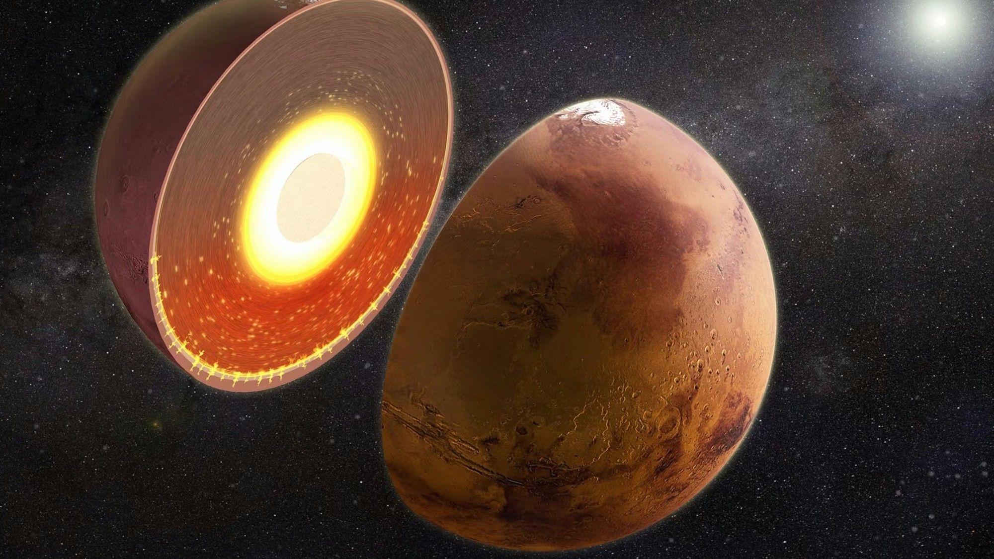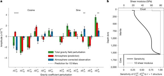
MainMars exhibits a prominent dichotomy in crustal structure. Whereas low-lying plains cover the northern hemisphere of Mars, the southern hemisphere is more topographically elevated, rugged and densely cratered16. These asymmetries potentially accompany an approximately 25 km mean variation in crustal thickness11 (or a roughly 200 kg m−3 variation in crustal density17,18), as well as spatial differences in crustal magnetization19 and seismic wave attenuation20. The northern lowlands may also have held surface water before the loss of Mars’s putative oceans to space21. Understanding the origin of the crustal dichotomy of Mars therefore constrains the planet’s ancient hydrology and the timing of surface conditions capable of supporting life22.The origin of the hemispheric crustal dichotomy of Mars is widely debated. Some studies suggest that a giant impact disrupted the primordial mantle of the planet and either thickened the crust across the southern hemisphere23,24 or excavated the northern hemisphere25. Other studies suggest that mantle convection over one hemisphere drives subsidence and resurfacing of the northern crust or thickening and uplift of the southern crust12,13. These formation hypotheses for the crustal dichotomy predict long-lived structures within the Martian deep interior that may persist into the present day12,13,23,24. For example, crustal thickening over the southern hemisphere could enhance thermal insulation and radiogenic heating of the deeper interior, resulting in a structurally weak underlying mantle14,15. Here we investigate the character of these potential heterogeneities at depth by analysing the gravitational response of Mars to seasonal (that is, 687 Earth days) tidal interactions with the Sun.The Martian gravity field can be expressed in terms of spherical harmonic coefficients of degree ℓ and order m (Cℓm and Sℓm), with the full wavelength at a given ℓ usually defined as roughly 2πR/ℓ (R = 3,396 km)26. Temporal variations can be modelled as cyclic perturbations to these coefficients and separated into in-phase (or ‘cosine’, A) and (a quarter cycle) out-of-phase (or ‘sine’, B) components over a given period (that is, \(\Delta {C}_{{\ell }m}^{A,B}\) and \(\Delta {S}_{{\ell }m}^{A,B}\)) (Methods). For a spherically symmetric planet, forcing at a given degree and order excites deformation only at the same degree and order. In this case, tidal forcing acts almost entirely at degree-2 and will contribute negligibly to the gravity field of Mars at higher degrees (that is, \(\Delta {C}_{3m}^{A,B},\Delta {S}_{3m}^{A,B}\approx 0\)). However, lateral heterogeneity in the internal structure of Mars (for example, north–south variations in shear modulus) can couple with degree-2 forcing to produce substantial degree-3 signals such that \(\Delta {C}_{3m}^{A,B},\Delta {S}_{3m}^{A,B}\ne 0\) (ref. 8). Moreover, although static gravity fields carry some sensitivity to deep-seated density structure (especially at long wavelengths), their sensitivity is weighted towards structure in the shallower interior at all degrees (equation (4) of ref. 27). By contrast, the low-order non-zonal (that is, m ≠ 0) time-variable gravity field of Mars is most sensitive to lateral variations in the shear modulus of the mantle, as these heterogeneities generate larger mass redistributions than comparable perturbations within shallower layers4,9. Measuring time-variable gravity signals (for example, by analysing the trajectory of orbiting spacecraft) correspondingly provides a direct means to constrain the extent of Mars’s deep-seated heterogeneities4.Measuring the seasonal tidal response of MarsTo recover the seasonal degree-3 tidal signals of Mars, we analyse Earth-based X-band Doppler tracking data acquired by the NASA Deep Space Network (DSN) from several Martian orbiters. We use radio science data from MGS, ODY and MRO spanning a total of 16 years. Our data processing procedure follows the approach used to determine the time-varying zonal (m = 0) gravity field of Mars in ref. 28 but is extended in this study to include non-zonal ℓ = 2 and ℓ = 3 time-varying gravity field coefficients over the seasonal (or annual) 687-day period.Recovered non-zonal degree-3 gravity field coefficient perturbations are presented in Table 1 (for zonal and degree-2 coefficients, see Extended Data Table 1). To account for modelling uncertainties, particularly those arising from unmodelled non-gravitational accelerations, we inflate the formal uncertainties of these coefficients by a factor of 15 (see, for example, ref. 4) in Table 1 and in all subsequent analysis. As in ref. 28, we directly model the effects of the atmosphere by integrating the impact of the Mars general circulation model on gravity coefficients (Methods and Extended Data Figs. 1 and 2).Table 1 Recovered degree-3 non-zonal time-varying gravity field for Mars with 15× formal uncertaintiesFull size tableModelling the mantle structure of MarsWe recover non-zonal ℓ = 3 perturbations to the Martian gravity field that deviate substantially from values predicted for a spherically symmetric Mars with an atmosphere (Fig. 1a). For example, the cosine coefficient of the ℓ = 3, m = 1 gravity field perturbation (that is, \(\Delta {C}_{31}^{A}\)) deviates approximately 300% from expectations for a spherically symmetric Mars with atmospheric loading (with >99.99% confidence, the difference between the green and red bars in Fig. 1a), suggesting coupling between tidal deformation and laterally heterogeneous internal structure in the mantle of Mars (Fig. 1b). To constrain the nature of these asymmetries, we perform a Bayesian, Markov chain Monte Carlo inversion (Methods). Inversions incorporate both degree-2 and degree-3 (zonal and non-zonal) time-variable gravity fields of Mars as constraints (Table 1, Extended Data Table 1 and Methods).Fig. 1: Sensitivity of the Martian seasonal gravity field to laterally heterogeneous structure.a, Bar chart showing the amplitude of seasonal temporal variations in selected Martian ℓ = 3 gravity field coefficients (that is, \(\Delta {C}_{3m}^{A,B}\) and \(\Delta {S}_{3m}^{A,B}\), in which A and B denote cosine and sine terms, respectively). Green, red and blue bars, respectively, denote the median total gravity field perturbations, the predicted median impact of the atmosphere on perturbations and the median observed gravity field perturbations corrected for the atmosphere. Error bounds on the green and blue bars represent 15× formal 1σ uncertainties and asterisks denote statistical significance of the atmosphere-corrected observation relative to the null hypothesis (that is, expectations for a spherically symmetric Mars with no atmosphere; amplitude = 0, the horizontal dashed line). **P < 0.01 and ****P < 0.0001 for two-tailed t-tests. Error bars on predictions for red bars are 1σ uncertainties computed by comparing inter-annual variations in the assumed atmospheric model (Extended Data Fig. 1). Error bars on atmosphere-corrected coefficients (blue bars) are generally much larger than (and therefore implicitly account for) uncertainties associated with inter-year variations in the Martian gravity field from our nominal atmospheric model (red bars) but do not directly consider the impact of extreme atmospheric models on coefficients (Methods and Extended Data Fig. 1). b, Normalized sensitivity of gravity coefficients to ℓ = 1 perturbations in shear modulus versus depth for Martian interiors subject to ℓ = 2 tidal forcing. The average shear modulus with depth assumed for Mars is plotted as a grey line for reference (Extended Data Table 2). Labels refer to vertical regions spanning the crust (0–50 km depth), the mantle (50–1,560 km) and the core (1,560–3,390 km).Our model space consists of lateral shear modulus variations imposed onto a 1D reference interior constrained by Mars’s degree-2 tidal Love number, moment of inertia and seismic travel-time data29 (Extended Data Table 2). We expand these variations in a spherical harmonic basis truncated at degree ℓ = 3 across two internal layers: the crust (0–50 km depth) and the mantle (50–1,560 km depth). Lateral crustal thickness and density variations on Mars negligibly (<0.3%) affect the time-variable gravity field and are therefore ignored for inversions. Heterogeneities in the core (including a potential solid inner layer30) also minimally affect time-variable gravity fields (Fig. 1b). We consequently prescribe a uniform elastic structure below 1,560 km depth. We use the semi-analytical spectral code LOV3D (ref. 10) to forward compute coupling between degree-2 forcing and lateral heterogeneity for candidate interior structures (Methods). Note that the zonal gravity field variations of Mars are also sensitive to seasonal CO2 condensation over the polar caps31. We accordingly model m = 0 terms as the sum of the solid-body tide and a seasonal mass exchange of 6.2 × 10¹⁵ kg and 8.4 × 10¹⁵ kg over the northern and southern polar caps, respectively28 (Methods).Our results indicate that degree-1 (ℓ = 1) shear modulus structure, which reflects a hemispheric pattern, enhances the amplitude of ℓ = 3 coefficients for Martian interiors subject to seasonal tidal forcing at ℓ = 2 (Fig. 1b). For example, the ℓ = 2, m = 1 harmonic associated with the obliquity tide of Mars interacts with north–south (that is, ℓ = 1, m = 0) shear modulus structure (lower/higher shear modulus values in the mid-latitudes of the southern/northern portions of the meridional hemisphere that spans −90° E to 90° E longitude) to regionally increase/decrease outward radial deformation. The resulting mass displacement yields an ℓ = 3, m = 1 gravity signature that enhances the amplitude of \(\Delta {C}_{31}^{A}\). Interaction between other hemispherical variations such as east–west (ℓ = 1, m = −1) and meridional (ℓ = 1, m = 1) asymmetries and the full degree-2 Martian tide (that is, components arising from both obliquity and eccentricity of Mars) is more complex10 but produces deviation of several degree-3 gravity coefficients from zero (Extended Data Fig. 3). By contrast, the degree-2 time-variable gravity field does not measurably deviate from predictions for a spherically symmetric interior (Extended Data Fig. 3), suggesting minimal internal heterogeneity that strongly couples with ℓ = 2 forcing10 (for example, ℓ = 2 patterns; Extended Data Fig. 4).Our inversions predict statistically significant degree-1 variations in the shear modulus of the Martian mantle. Specifically, we resolve north–south, meridional and east–west patterns with peak-to-peak amplitudes (and 3σ uncertainties) of 60 ± 40%, 42 ± 38% and 36 ± 34%, respectively (Fig. 2a–c), as well as an overall variation of 81 ± 60% (or >20%). Inversions fit all time-variable gravity field constraints to within 3σ uncertainty (Extended Data Fig. 3) and do not recover any statistically significant lateral variations in shear modulus for the crust of Mars (Extended Data Table 3 and Extended Data Fig. 4a) or for degrees higher than ℓ = 1 in the mantle (Extended Data Table 3 and Extended Data Fig. 4b). Note that heterogeneity amplitudes represent averages over the entire mantle depth range. This averaging is necessary to produce statistically significant results, because the sensitivity of degree-3 time-variable gravity to 3D structure varies gradually with depth (Fig. 1b), resulting in substantial non-uniqueness between recovered heterogeneity amplitudes when the mantle is subdivided into several layers (Extended Data Fig. 5). Even so, our inversions do not necessarily preclude more vertically localized structure within the mantle of Mars (for example, at the base of the lithosphere14 or near the core–mantle boundary32).Fig. 2: Tidal tomography of the Martian mantle.a–c, Histograms of inverted coefficient values that describe internal hemispheric (degree-1) variations in shear modulus (in per cent relative to the bulk value) for the Martian mantle (50–1,560 km depth). Meridional (a), north–south (b) and east–west (c) labels denote order-1, order-0 and order-1 variations, respectively. Dotted lines indicate 0.3rd and 99.7th percentiles (that is, 3σ confidence bounds) and the solid red lines indicate maximum a posteriori solutions (that is, the location of the absolute maximum of posterior distributions). A full list of derived harmonic coefficients describing 3D structure is shown in Extended Data Table 3. d, Plot of Martian topography (MGS-M-MOLA-5-IEGDR (ref. 54), red–orange–yellow–green–blue colour map) overlain by semi-transparent map of the combination of maximum a posteriori solutions for degree-1 variations in mantle shear modulus shown in a–c (red–blue colour map). Black contour indicates the trace of the zero value of shear modulus variations. Approximate locations of Tharsis, Vastitas Borealis and Hellas basin are indicated. Map is shown in Mollweide projection.The hemispheric mantle shear modulus variation of Mars broadly matches the spatial pattern of the crustal dichotomy (Fig. 2d). For example, combining maximum likelihood solutions for recovered degree-1 order-1, order-0 and order-−1 variations (Fig. 2a–c) results in a region of increased shear modulus beneath the northern lowlands (centred at 45° N, 138° W over Vastitas Borealis; Fig. 2d) and a corresponding reduction in shear modulus beneath the southern highlands (centred at 45° S, 42° E near Hellas basin; Fig. 2d). The zero-value contour of the mantle shear modulus variation of Mars also tracks the boundary of the crustal dichotomy, including its southward (or northward) deflection over the anti-meridional (or meridional) hemisphere. The correspondence between surface geology and mantle stiffness variations weakens between 40° W and 139° W near the volcanic Tharsis rise region, potentially because of overprinting of the dichotomy boundary by this structure16. The lack of anomalies observed directly beneath Tharsis (Fig. 2d) also suggests that present-day internal structures associated with this feature are small in amplitude (that is, compared with asymmetries in Fig. 2), shallow or restricted to a relatively small (ℓ > 3) lateral region within the interior33.Thermal anomaly beneath the highlands of MarsOur modelling suggests that the anomalous degree-3 gravity field of Mars arises owing to a substantial, >20% lateral variation in the mantle’s effective shear modulus at the seasonal timescale. What could generate such a large contrast? At a given pressure, the rigidity of mantle rock depends on both temperature and composition. At seismic timescales, crystalline temperature differences would need to exceed an unrealistically large >1,000 K to produce observed shear modulus variations4. However, when extended to the Martian annual period (Methods and Extended Data Fig. 6), the effective shear modulus of olivine becomes approximately 15–20 times more sensitive to temperature34. As such, recovered shear modulus variations can mostly be explained by a hemispheric temperature anomaly of approximately 200–400 ºC in the present-day Martian mantle (Fig. 3 and Methods). Thermal modelling also suggests that the insulating effect of the thicker crust in the southern highlands can result in a hemispheric temperature contrast >200 ºC (Fig. 3f of ref. 15), consistent with our results. The centre-of-mass–centre-of-figure (COM–COF) offset of Mars also limits the potential compositional component (for example, iron, water content) of asymmetries because, in isolation, such differences (and their associated density structure) would need to produce an offset that is approximately 50 times larger than observations35 to account for the inferred shear modulus variations. Even so, our models allow for up to 5% iron enrichment (that is, variation in forsterite–fayalite mole fraction or ΔFo–Fa) within the mantle of the southern highlands (Fig. 3).Fig. 3: Relationship between temperature, composition and inferred shear modulus variations in the Martian mantle.Shaded regions indicate the constrained ranges of the inferred Martian effective hemispheric shear modulus variation and the impact of mantle structure on the COM–COF offset as a function of southern highlands mantle temperature anomaly and fayalite–forsterite mole fraction contrast (Fa–Fo) (for details on calculations, see Methods). Values are projected onto a degree-1 pattern with poles centred at 45° N, 138° W (northern lowlands) and 45° S, 42° E (southern highlands). Black contours indicate COM–COF offsets at 10-km intervals. Because the COM–COF offset is sensitive to the structure of both the crust and the mantle, our modelled 0–1.31-km range of values accounts for the possibility of: (1) an anomalous COF that is fully attributable to elevated topography over the southern highlands (paired with Airy or Pratt compensation of this structure at depth) or an anomalous COM arising from a relatively dense crust over the northern lowlands (that is, the 0 km bound)11,18,35; (2) an anomalous COM that is only attributable to mantle density variations (that is, the 1.31 km bound); and (3) intermediate cases. The grey-shaded area and thick solid black line, respectively, denote the 99.7% confidence bounds and preferred value for the overall shear modulus difference of 81 ± 60% inferred from gravity data in this work (Fig. 2). By identifying overlapping portions of parameter space that satisfy both the 99.7% range of inferred shear modulus variation and COM–COF offset, we infer that hemispheric asymmetries can be explained by a temperature anomaly of 200–400 ºC and an iron enrichment of up to 5% in the southern highlands mantle.Mantle heterogeneities may preserve signatures of, and thus provide independent constraints on, geodynamic processes that influence the evolution of the crustal dichotomy. We consider three such candidate processes: a giant impact, spontaneous degree-1 upwelling (that persists into the present day) and enhanced thermal insulation or radiogenic heating of the southern highlands mantle by a thick overlying crust. Spontaneous degree-1 upwelling or thermal insulation would produce a mainly thermal mantle anomaly12,13,14,15 as well as potential secondary compositional signatures through decompression melting below the lithosphere12,13,14,15. However, enhanced melt extraction in these scenarios would deplete the southern highlands mantle in iron12,36, opposite to the observations (Fig. 3). By contrast, a giant impact is (in isolation) not expected to result in a long-term secular variation in temperature of several hundred kelvin over a given hemisphere37. A hybrid scenario could resolve this mismatch. For example, following the formation of the northern lowland crust from the Borealis impact, the northern hemisphere mantle is first depleted in iron36, leaving the southern mantle relatively enriched. The resultant thicker southern crust could also trigger preferential thermal insulation15 or degree-1 upwelling38 below the highlands of Mars (the latter would be favoured absent variations in crustal thickness or radiogenic material abundance18), increasing the present-day temperature of this region (Figs. 3 and 4).Fig. 4: Conceptual model of the interior structure of Mars as inferred in the present study.Measured temporal variations in degree-3 gravity indicate a thermal anomaly within the mantle beneath the southern highlands (light yellow to orange regions outside the core). This anomaly may promote partial melting below the lithosphere of Mars, which ascends and stalls in the crust before reaching the surface14. This upwelling could result in thickening and enhanced magnetization across the southern highlands crust of Mars. By contrast, the mantle beneath the northern lowlands is comparatively cool (dark red to brown regions). Illustration is not to scale.Temperature variations may also influence the dissipative properties of the mantle of Mars. For example, comparisons of low-frequency marsquakes detected by the InSight (Interior Exploration using Seismic Investigations, Geodesy and Heat Transport) lander indicate substantially lower quality factors (Q ≈ 500) for events originating in the nearby Terra Cimmeria region of the southern highlands than for events from Cerberus Fossae in the northern lowlands (Q ≈ 800–2,000)20. These differences in attenuation can be attributed to lateral variations in the temperature of the mantle of a few hundred kelvin (Fig. 4 of ref. 20). A warm southern highlands mantle might also result in localized melting14, which could reduce the 200–400 ºC temperature anomaly required to explain gravity field observations (Fig. 3). However, the Q values inferred for the southern highlands remain well above those expected for partially molten olivine (Q ≈ 100 or lower)20. Even so, future electromagnetic sounding measurements (for example, ref. 39) could resolve whether the inferred thermal anomaly in the southern highlands mantle is associated with isolated magma pockets or with a more continuous molten layer at depth (for example, refs. 14,32).The preferential magnetization of the southern highlands crust19 may also reflect the effects of a laterally heterogeneous interior. For example, upwelling beneath the southern highlands may have heated the overlying crust above Curie temperatures while Mars’s ancient dynamo was active (4.5–4.1 billion years ago)40. These temperatures may have subsequently fallen below Curie temperatures before the cessation of the dynamo, allowing affected portions of the southern highlands to acquire their present-day remanent magnetization13,41. Alternatively, increased heat flow at the core–mantle boundary (and in the overlying mantle) may have regionally enhanced convection in the outer core of Mars, resulting in a stronger dynamo below the southern highlands42. Inferred asymmetries in mantle structure may therefore constitute a present-day remnant of geodynamic processes associated with the generation of Mars’s early dynamo (Fig. 4).Volcanism and future measurementsAlthough melt is not required by our results (Fig. 3), some thermal models predict that higher temperatures in the southern highlands mantle would increase magma production in this region14. Such pockets of deep-seated melt are expected to ascend and erupt onto the surface over timescales of several Myr (ref. 43) (Methods). Yet recent (tens of Myr) volcanic activity is confined to Cerberus Fossae in the north44. We propose two potential solutions to this apparent paradox. The first is that the thicker (and potentially lower-density45) crust in the southern highlands may present a barrier to melt ascent. Under this scenario, melt would stall in the mid-crust and generate local intrusive features (Fig. 4). These intrusions would be difficult to detect in surface images but may be resolved from very-high-resolution (ℓ > 300) measurements of the static gravity field of Mars46. The second solution is that melt ascent and eruption requires a background extensional stress field47. Tectonic features in the southern highlands are dominantly compressional (for example, ref. 48), as expected from the slow cooling of Mars. By contrast, Cerberus Fossae is a region undergoing localized extension49. In any case, the petrology of volcanic rocks sampled from different locations over the crust of Mars could constrain the spatial differences in mantle potential temperature implied by our results50.Tidal tomography—or the inference of lateral variations in interior structure from a body’s time-variable response to tidal forcing—has been used to investigate the mantle of Earth2 and, more recently, the Moon4. Here we use nearly two decades of precise spacecraft tracking data to extend this approach to Mars. Future missions with dedicated gravity experiments (similar to GRACE for Earth51 or GRAIL for the Moon52) could resolve similar (or finer) variations in Martian mantle structure over much shorter mission durations53. In the future, these techniques may also be applied to other planetary bodies that exhibit pronounced low-order asymmetries in structure, including Ganymede, Mercury, Io and Enceladus. Because tidal tomography largely relies on remote measurements, it represents a powerful tool for future missions seeking to characterize the interiors of planetary bodies without landed spacecraft.MethodsModelling the time-varying gravity fieldThe gravitational potential for Mars, U(r, λ, ϕ), can be expressed as a sum over 4π-normalized spherical harmonic coefficients Cℓm and Sℓm: $$U(r,\lambda ,\phi )=\frac{{GM}}{r}\left[1+\mathop{\sum }\limits_{{\ell }=2}^{{\rm{\infty }}}{\left(\frac{{R}_{m}}{r}\right)}^{{\ell }}\mathop{\sum }\limits_{m=0}^{{\ell }}({C}_{{\ell }m}\cos m\lambda +{S}_{{\ell }m}\sin m\lambda ){P}_{{\ell }m}(\sin \phi )\right],$$
Tidal tomography reveals a thermal anomaly beneath Mars’s crustal dichotomy - Nature
Analysis of tracking data from Mars orbiters reveals time-variable gravity field behaviour reflecting the structure underlying the Martian crustal dichotomy and indicates the preservation of a 200–400 °C thermal anomaly in the present-day mantle below the southern highlands.
11,715 words~53 min read