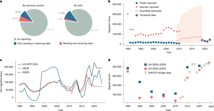
MainThe movement of people—within countries and between them—is an important topic across multiple domains. Migration drives demographic change, shaping the size and composition of populations; it can influence labour markets1, inform social policy2 and is a popular topic for public debate3. Although migration often follows long-term trends driven by development4, it can be dramatically altered by short-term shocks—armed conflict, famine, natural disasters, political instability, changes in national borders, peace agreements or independence movements5.Human migration, however, is notoriously difficult to define and track6. Current analyses of global migration systems rely heavily on migrant population data published at five-year intervals by the United Nations (UN) and at ten-year intervals by the World Bank. These datasets provide counts of migrants in each country by country of birth, typically referred to as stock data. Although relatively straightforward to collect, they offer only a snapshot at a fixed point in time and provide limited insight into the temporal dynamics of migration: migrants may have arrived immediately before the observation point or several decades earlier. To better capture migration dynamics, researchers have developed methods that estimate migration flows over multi-year periods by comparing changes in migrant stocks at the beginning and end of each interval9. However, as these estimates are tied to gaps in the underlying stock data, the resulting five- or ten-year estimates inevitably smooth or completely miss movements that occur in the intervening years. What researchers on global migration ideally need are annual flow data for all countries. Such data would allow them to track the tempo of migration systems with far greater precision, integrate migration patterns with other annually reported datasets on drivers such as economic change, conflict, climate or policy reforms, feed into annual population projection models, and facilitate both causal and comparative analyses across countries and regions. Yet existing annual migration flow data are predominantly available only from high-income Western countries with the statistical infrastructure to monitor migration. Such data only cover a small share of the global migration system7,8 (Fig. 1a) and reinforce a receiving-country bias in global migration research15.Fig. 1: Availability of flow data across global migration corridors.The alternative text for this image may have been generated using AI.Full size imagea, Fraction of corridors that have reported flow values in the 1990–2020 period by any of the validation datasets used in this work7,66,67,68,69. Statistics for both origin- and birth-destination corridors are shown; these are further disaggregated by corridors for which neither, only one of, or both the sending and the receiving country has reported figures. b, Migration flow estimates based on domicile registration (usually with a local authority) are available for a small number of countries, but the discrepancies can be large: estimates of flows—based on registrations of people arriving from Poland as reported by German authorities (red) and de-registrations of people leaving Poland for Germany, as reported by Polish authorities (blue)7—are shown. The harmonized QuantMig estimates (orange; error bands show the 97.5% quantile) and the recent digital-trace estimates based on Facebook data are also shown. c, Various estimates of the net migration for France, such as those from the UN Population Division’s World Population Prospects (2024 Revision), the US Census Bureau (USCB)’s International Dataset70, and the French National Institute of Statistics and Economic Studies (INSEE)71. d, UN DESA estimates of the migrant stock of Somalians in Ethiopia, which do not agree across revisions. In some cases, they are based on refugee data figures from the UNHCR72.In countries in which migration flow statistics are published, the definitions of what constitutes a migration event are determined by criteria designed to meet domestic policy needs16,17, which can bias comparative analyses. Although the UN recommends a twelve-month threshold18, where anyone relocating for the majority of a year or more qualifies as a migrant, this definition is not applied consistently. Some countries such as Germany mandate residential registration, requiring migrants to report their country of origin upon arrival. Others, such as the UK, rely on visa records, administrative data and, until recently, passenger surveys. A third common approach uses border entry statistics collected by immigration authorities. Each method has limitations: registration systems typically undercount emigration, as few individuals de-register when leaving; passenger surveys and border data are not comprehensive and may conflate short- and long-term travellers. As a result, estimates from sending and receiving countries often diverge markedly. For instance, in 2005 Germany reported 160,000 arrivals from Poland, whereas Poland recorded only 12,300 departures to Germany (Fig. 1b). In Europe, to reconcile such discrepancies, statistical demographers have developed models to estimate bilateral migration flows between countries. The most recent study, the QuantMig project10,11, made use of a Bayesian framework alongside expert insights to estimate bilateral migration flows for 30 European countries from 2009 to 2019. This produced a harmonized dataset, revealing substantial uncertainty—in some cases, with credible intervals spanning over 100%. Given the dearth of migration flow statistics available to monitor many major migration corridors between developing countries, this approach does not easily generalize to a global environment. Labour migration data represent another important source19, as migrant workers often make up a substantial share of international movers. However, here too definitions and data standards vary widely between countries20, and undocumented migration—by its very nature—remains largely invisible to official statistics.A recent study attempted to bypass official data sources for monitoring global migration flows by analysing digital traces21. By monitoring changes in aggregated, anonymized monthly Facebook location data to estimate bilateral flows among 181 countries between 2019 and 2022, the study captured, for example, the displacement of Ukrainians following the Russian invasion, the Venezuelan migration crisis and altered migration patterns during the pandemic. The digital traces from more than three billion users were weighted to represent population-level migration flows, accounting for differences in Facebook usage and economic development along each corridor, and calibrated against official migration statistics in selected countries. These data provide, for the first time, a near-global direct estimate of migration flows.One macroindicator that many countries are interested in estimating is the net migration—that is, the balance of immigration and emigration. A small number of countries publish net migration figures, estimated from immigration and border statistics (Supplementary Fig. 1), whereas on a global scale, the UN Department of Economic and Social Affairs (UN DESA) provides figures from 1950 onwards in its World Population Prospects (WPP) reports. These are primarily based on demographic estimates rather than migration statistics. As births and deaths are more widely and consistently tracked than migration figures, in principle the net migration can be estimated by subtracting the natural change (births minus deaths) from the total population change. Although this approach is theoretically sound, in practice it is hindered by irregularities in measuring the total population and its change over time, which are sensitive to inconsistencies in census methodology. Consequently, demographic net migration estimates can differ noticeably from migration-based statistics, even for countries whose population data are of high quality (Fig. 1c).Here we combine deep learning with a mechanistic flow model to estimate annual bilateral migration flows in the 1990–2023 period between all 230 countries and regions recognized by the UN. Our data are disaggregated by country of birth, meaning that, aside from the flows and the net migration for each country, we also obtain a complete dataset of annual migrant stocks, that is, the number of migrants Sbj(t) born in country b residing in country j in year t. A deep neural network is trained on an extensive set of socio-economic and cultural covariates for each country (Extended Data Table 1), allowing us to disentangle the drivers of migration and opening the door to future forecasting of migration flows. The network is trained to match a set of target data, comprising the UN DESA migrant stocks22, Facebook data, as well as a small number of predominantly European bilateral flows and net migration data. The target data are used to construct a loss function, which is iteratively minimized during training23,24. The loss function quantifies the mismatch between predictions and targets, and is an objective that the neural network seeks to minimize by following the loss gradient, or direction of steepest descent. Once trained, the neural network acts as a function mapping input covariates to migration flows (Extended Data Fig. 1). By training a family of neural networks and further ‘pushing’ the uncertainty on the input data through the network, our approach also enables uncertainty quantification, allowing us to pinpoint the countries in which data are inconsistent and collection should be improved.This marks a paradigm shift for the computational toolset hitherto used to model global migration. Most past techniques have relied solely on migrant stock data published by UN DESA, which provides estimates at five-year intervals from 1990 (Fig. 1d). The simplest estimation techniques are based on stock differencing9 and assume that the bilateral flow Fij is equal to the difference in stocks Sbj(t + 1) − Sbj(t) with b = i. Negative differences are either dropped (meaning zero flow)25,26 or counted towards flows in the opposite direction27. The simplifying assumption here is that bilateral migration flows only take place from a person’s country of birth to a destination; that is, the stock of Swedes in the UK changes only due to Swedish people arriving from and returning to Sweden; but not due to Swedish people arriving from, say, Norway. To account for this, a more sophisticated array of so-called demographic accounting methods were proposed12,13,14. These attempt to infer a three-dimensional flow matrix Tbij, with each entry modelling the flow of people born in b moving from i to j, allowing for greater flexibility, but also greatly increasing the number of parameters to be estimated. The flow table is constrained such that its estimates reproduce the stock differences. These are typically first adjusted to account for births and deaths, whereby the estimated flow reproduces only the change in stocks not caused by demographic change.Stock-based flow estimation approaches all take the stock data at face value; they are also unable to increase the temporal resolution of the estimates, and have thus far only yielded five- or ten-year flows (the resolution of the UN DESA or World Bank data). An alternative is the use of gravity models28, broadly taken to refer to any type of regression-based approach that relates the flow to a set of covariates χ. These models can, in principle, capture flows at any resolution, provided the covariates are of sufficient quality and are suitably chosen; however, they tend to perform poorly when modelling migration29, even with a large and sophisticated set of covariates. The fundamental problem when modelling migration as $$\log {T}_{bij}(t)=f({\chi }_{bij}(t))$$is that it represents humans as Markovian, acting only on the basis of the current state of the world with no regard to the past. This may be warranted when considering the response to a sudden, cataclysmic event, but is hardly reasonable when incorporating long-term, macro-level political, economic or social indicators. The decision to leave is, in most cases, not merely predicated on the current economic climate: crises from past years can influence a person’s decision, due to a multitude of delayed effects and complex feedback loops. Any model that does not account for the system’s memory will thus fail to accurately reproduce, let alone explain, the temporal and spatial variance in human migration. Here we use a recurrent neural network30,31, which implements a form of ‘memory’ by maintaining a ‘hidden’ or ‘latent’ state z(t) that changes over time. This allows the network to selectively retain past information using a dynamic filter and learn temporal correlation patterns of varying length. The latent state incorporates past dynamics to inform the flows of today without assuming temporal stationarity in migration flows, which are typically unstable32.In recent years there has been a steep increase in the application of machine learning methods to predict and explain human migration and mobility patterns33,34,35. Studies have applied machine learning methods, including deep learning approaches, in a multitude of settings. Most applications have been developed to address commuting and mobility patterns within cities, regions and countries36,37,38,39,40. Modelling efforts in migration research have largely focused on internal moves within countries41,42,43, including analyses of climatic and environmental drivers of mobility44,45,46,47, as well as forecasting asylum seeking and irregular international migration into predominantly high-income Western states48,49. Unlike in the global migration data setting, movement response variables in this recent literature have been derived from a single source, where the challenges of combining measures and the problems of missing or inconsistent data across multiple origin-destination corridors are absent. Furthermore, rather than quantifying the scale and patterns of international migration at the global level, the focus of these studies has been on providing superior extrapolatory predictions to classic modelling approaches or on helping detect possible linkages between covariate factors and mobility or migration in data-rich settings.The article is structured as follows: first, we present the estimation results, showcasing the data on a selection of case studies. We validate our method’s performance on test data of unseen flows and compare it with a selection of standard methods discussed above. The inference method is presented in detail in the Methods. We denote the stock estimates as S, the flows disaggregated by birth as T, the total origin-destination flows as F and the net migration as M. For notational clarity, we will omit the time argument wherever possible. Estimated quantities will be denoted by a hat, for example, \(\hat{{\bf{M}}}\).A global map of migrationOur estimates reveal that, since 2000, global migration movements have risen from 13 million people annually to around 35 million in 2023 (Fig. 2a). This trend is not explained by a rising global population, as per-capita migration saw a similarly steady increase from 0.2% in 2000 to 0.45% in 2023 (Extended Data Fig. 2). Since the turn of the millennium, total global migration has only seen two periods of sustained decrease: during the Great Recession in 2008 to 2009, and during the COVID-19 pandemic in 2020. The largest single-year event we registered is the 1994 movement of people from Rwanda to the Democratic Republic of the Congo, totalling almost 950,000. Globally, the Middle East experienced the highest total inflow of migrants, chiefly from South Asia and the Philippines, with immigration from Bangladesh to Saudi Arabia alone averaging around 300,000 people per year from 2010 onwards (Fig. 2c). We estimate that, since 2010, a total of 19 million people, averaging 1.35 million per year, migrated from India, Pakistan and Bangladesh to Saudi Arabia, Qatar, Bahrain and the UAE—this compares to 13.6 million movements from Mexico to the USA over the entire period since 1990.Fig. 2: Global bilateral, annual migration flows, disaggregated by country of birth, for all countries and territories from 1990 to 2023.The alternative text for this image may have been generated using AI.Full size imageError bands indicate the mean and one s.d. over n = 1,500 samples from the neural network ensemble. Regions in this and the following panels have been selected to cover a diversity of country sizes, income levels and geographies. a, Total global flows, in millions. The increase cannot be explained by the rising global population, as the per-capita figures show a similar trend (Supplementary Figs. 25 and 26). b, Chord diagrams of regional flow patterns for 1990 and 2023, in millions. The arrow head indicates the direction of the estimated migration flow. The width of the arrow at its base indicates the size of the migrant flows. Numbers on the outer section axis indicate the size of the migration flows, in millions. The axes are fixed on the scale of the sum of the regional immigration and emigration flows in 2023 for direct comparisons between years. Colours correspond to the countries’ region of origin. c, The six largest country-level flow corridors of the past 35 years, measured by total flow in millions. Facebook data are also shown.Europe consistently ranks as the region with the highest volume of intraregional migration, surpassed only once by sub-Saharan Africa in the early 1990s during the Rwandan civil war (Extended Data Fig. 3). Pre-2020, gross flows in Europe reached around three million people annually, having steadily increased during the 2000s and 2010s following the eastward expansion of the EU and the Schengen region. Flows from Eastern to Western Europe since 1990 total around 20 million, or 600,000 per year. Figure 3 shows a snapshot of intra-European flows in 1991, following the collapse of the Soviet Union, colour-coded by country of birth. In that year, by our estimates, intra-European flows reached about 2.02 million people, of which 807,000 alone were of people born in Poland, Russia, Ukraine and Romania. The largest movements took place between Ukraine and Russia, Kazakhstan and Russia, and into Germany. During this time, we see high levels of return migration (bidirectional movement), as some sought to return to their country of birth, whereas others relocated abroad in search of economic opportunity. Figure 3b shows the flow estimates \(\hat{F}\) for a selection of corridors, alongside values from the various datasets used to train the neural network. Our estimates match not only the data, but also the uncertainty on the QuantMig values exceedingly well (refer below the discussion on uncertainty quantification).Fig. 3: Migration in Europe.The alternative text for this image may have been generated using AI.Full size imagea, Intra-European flows in 1991, colour-coded by country of birth. Some reference flows are indicated for scale. b, Total bilateral flows for selected European corridors. The estimates from the various target datasets used to train the model are also shown (Methods). Error bands represent the mean and one s.d. over n = 1,500 samples from the neural network ensemble.Migration in the Global SouthEurope is perhaps the region with the least need for a detailed analysis of migratory patterns, given that data are (relatively) plentiful. The value of our dataset lies primarily in what it tells us about movements in other parts of the world, especially the Global South. In the mid-2010s, for instance, sub-Saharan Africa saw several large-scale migration events. Civil war raged in the newly independent country of South Sudan from 2013 onwards, causing a large exodus into neighbouring Ethiopia (Fig. 4). The UN High Commissioner for Refugees (UNHCR) classifies the entire migrant population of South Sudanese in Ethiopia as refugees. Violence also erupted in West Africa, with the jihadist group Boko Haram starting an armed insurgency against the Nigerian government in 2009, and dramatically escalating its attacks in 2014, including by abducting nearly 300 young women from a school50,51. In 2013 to 2014 alone, we estimate that around 79,000 persons born in Nigeria moved or fled to neighbouring Chad, Niger, Cameroon—the majority of whom moved (45,000) to Niger. From 2009 to 2019, we estimate an outflow of Nigerian-born persons to these three countries of 250,000 with a s.d. of 31,000. This figure is dwarfed by the International Organization for Migration (IOM) estimate of around 2.4 million internally displaced people as a consequence of the violence52. Meanwhile, the ongoing civil war in the Central African Republic led to a continuous outflow to neighbouring Cameroon, Democratic Republic of the Congo and Chad.Fig. 4: Migration in sub-Saharan Africa.The alternative text for this image may have been generated using AI.Full size imagea, Flows in 2014, colour-coded by country of birth. Some reference flows are indicated for scale. b, Migrant stocks for selected country pairs. Error bands indicate the mean and one s.d. over n = 1,500 samples from the neural network ensemble. Refugee figures from the UNHCR, and UN DESA stock data with estimated uncertainties, are also shown (Supplementary Fig. 3).Revising the UN figuresIn Fig. 5a we show the net migration figures \(\hat{{\bf{M}}}\) for selected countries alongside the estimates MWPP from the 2024 WPP report53. Our dataset provides a valuable correction to these figures, which, as mentioned in the introduction, are calculated from demographic residuals rather than migration statistics: $${{\bf{M}}}^{{\rm{W}}{\rm{P}}{\rm{P}}}(t)=\Delta {\bf{P}}(t)-({\boldsymbol{\beta }}(t)-{\boldsymbol{\gamma }}(t)){\bf{P}}(t),$$with P(t) the total population, and β and γ the crude birth and death rates, respectively. The variation in the WPP figures is often caused by anomalies in the population figures, which strongly affect the change in population ΔP and cause, for instance, Vietnam’s net migration to spike at approximately 2008, only to then fall back to zero in 2010. Although the UN figures would suggest positive migrant inflow to Russia since 1995, our estimates show that, in fact, Russian net migration turned negative around 2005—a trend only reversed by the displacement of Ukrainians in 2022.Fig. 5: Net migration estimates and comparison with UN WPP data.The alternative text for this image may have been generated using AI.Full size imagea, Net migration figures for selected countries, alongside the WPP estimate, in millions. Error bands represent the mean and one s.d. over n = 1,500 samples from the neural network ensemble. b, Correlation coefficient of our estimates with WPP figures. c, Median relative uncertainty (s.d. over mean estimate) on our estimates.Meaningful uncertainty quantificationIn Fig. 5b we show the correlation between our net migration figures and the most recent WPP estimates53. We see a strong positive correlation across the The Organisation for Economic Co-operation and Development (OECD; this is unsurprising as these countries make up much of the target data), as well as across parts of the African continent and Central Asia. Our estimates of Indian net migration broadly follow the WPP trend, but are less erratic; the exodus of workers to the Gulf states, commencing in 2003, is clearly visible. The net migration estimates for Nigeria, meanwhile, are among the most uncertain of our model predictions: in Fig. 5c we show the median relative error (s.d. over mean estimate) for all countries, noting that for Africa, especially sub-Saharan Africa, the uncertainty on the net migration is among the highest in the world. By contrast, uncertainty is relatively lower for European and other rich Western countries, owing to greater availability and higher quality of data as well as more stable migration regimes. The pronounced regional heterogeneity in uncertainty highlights the importance of improving data collection in under-resourced settings as a prerequisite for more precise migration estimates (Supplementary Fig. 6).Testing and validationWe validate our approach by testing how well the neural network can reproduce unseen data (the test data) using fivefold cross-validation: we split the flow corridors into five equally large sets, and train five randomly initialized networks on each set of four folds, using the last fold as the test set. Following a previous work9, we chiefly assess performance through correlation metrics rather than mean errors. This allows for meaningful comparisons across datasets with inconsistent migration definitions and accommodates possible constant biases in our estimates. Figure 6a shows that the neural network achieves 94% correlation on the training data, and 73% correlation on the test flows, with only a 4% increase in median relative error (recall that many flows come with considerable uncertainty, and can be small in magnitude, so such a high relative error is not surprising: after all, an estimate of ten for a flow value of five represents a 100% relative error). Although this is the correlation across the entire dataset, we can also examine the distribution of correlations along each corridor (Fig. 6b), finding that the neural network generally matches the correlation distributions of the training data on the test set. In Fig. 6c we compare the estimated uncertainty of our model with that on the QuantMig data for Europe, as well as our estimates of the stock uncertainty with global coverage. The predicted uncertainty on the flows matches the QuantMig values well, while producing generally higher levels of uncertainty on the stocks than obtained through the demographic accounting procedure outlined in the Methods.Fig. 6: Performance evaluation.The alternative text for this image may have been generated using AI.Full size imagea, Performance on training and test data. We test the prediction performance using fivefold cross-validation on the target flows. The left-most panel shows the distribution of correlations along flow corridors on the training points (left half of each violin) and test corridors (right half). The distributions for the various flow datasets making up the flow target data over all folds are shown. The two panels to the right show the true and estimated flow values on both training and test sets, with the colour indicating the relative error. We achieve a Pearson R correlation of 94% on the training flows, and 73% on the test flows. The median relative error (MRE) is also indicated (Supplementary Fig. 22). b, The estimated stock values against the DESA stocks. The Pearson R correlation and MRE are also shown. c, Comparison of the uncertainties on the estimates (y-axes) and the QuantMig flows (left) and DESA stocks (right). The uncertainties on the DESA stocks are themselves estimated via demographic accounting and scaling, as described above (Supplementary Fig. 3). The Pearson R correlation is also shown.We conducted further experiments to assess whether extensive migration data from high-income countries bias the inference of global flows (refer to Supplementary Fig. 23 and the discussion from there onwards). Approximately 20% of the training data consist of flows originating from or directed to Europe or New Zealand (Supplementary Fig. 6). When this subset was withheld, predictions for other regions remained stable, indicating that the model does not transfer dynamics specific to highly developed regions to the rest of the world. To examine whether temporal coverage induces region-specific path dependencies, we withheld all observations after 2015; the predictions in developing regions showed no significant change (Supplementary Fig. 23E).We further validate the neural predictions on an additional dataset of unseen bilateral flows and compare their performance with those of the various stock-based approaches outlined in the introduction. The datasets and evaluation metrics are summarized in the Methods and refs. 9,54, and broadly comprised bilateral origin- or birth place-destination flows for a small number of (mostly Western) countries. The neural network estimates significantly outperform all other stock-based methods (Extended Data Figs. 4–6); the only exceptions are the UN WPP net migration estimates, where the demographic accounting methods, by design, show a perfect correlation of 1; however, given the methodological issues related to the UN WPP net migration estimates, this is not necessarily desirable.Finally, we are interested in gauging how sensitive the model is to the various input covariates. To this end, we calculate the elasticity ν of each neural network in the ensemble along every covariate dimension, that is, the relative change induced in Tbij ≡ T by a relative change in the kth covariate: $${\nu }_{k}=| \frac{{\chi }_{k}}{T}\frac{\partial T}{\partial {\chi }_{k}}| =| \frac{\partial \log T}{\partial {\chi }_{k}}| | {\chi }_{k}| .$$
Deep learning four decades of human migration - Nature
A global annual migration-flow dataset (1990–2024) is produced using deep-learning models and diverse sources to estimate movements across 230 countries with improved temporal resolution, coverage and uncertainty estimates.
12,032 words~55 min read