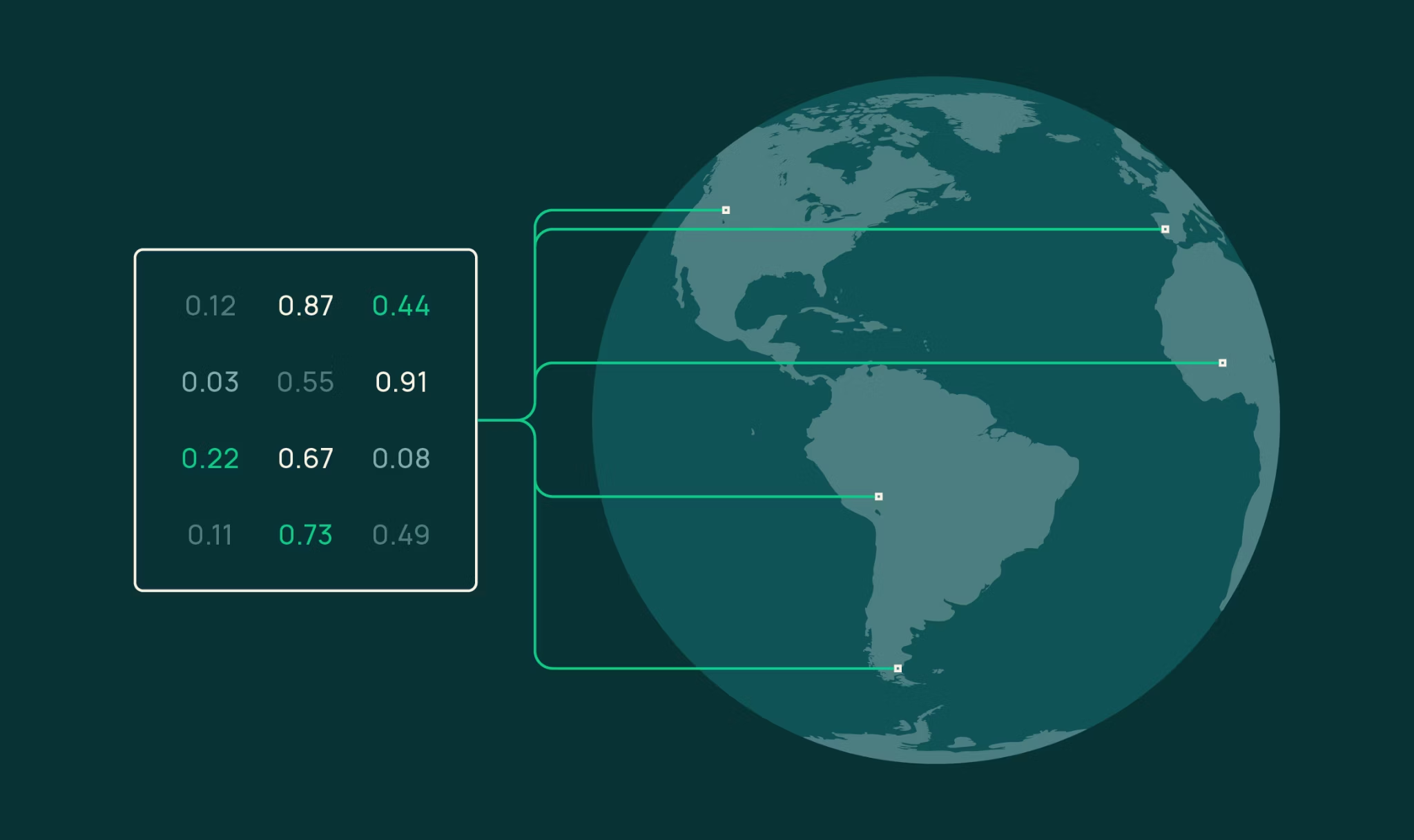
April 23, 2026Patrick Johnson, Favyen Bastani, Gabriel Tseng, Chris Wilhelm, Joseph Redmon, Hunter Pitelka, Patrick Beukema, Mike Jacobi, and Hadrien Sablon - Ai2Tech ReportDocumentationLearn more about OlmoEarthOlmoEarth Studio, our platform for building Earth observation models, now lets you compute and export embedding vectors—compact numerical representations of Earth-observation data produced by our open source OlmoEarth foundation models. The source code and model weights are publicly available alongside the research paper, so the community can inspect exactly how these embeddings are generated.Embeddings are a fast, cost-effective entry point for leveraging OlmoEarth: they support a wide range of downstream tasks, from similarity search to segmentation to unsupervised exploration. Locations with similar surface characteristics end up with similar vectors; locations that differ land far apart. OlmoEarth embeddings have shown strong performance in our own benchmarking and in independent evaluations. The exported Cloud-Optimized GeoTIFFs (COGs) are lightweight and easy to share. Choose your area of interest, time range, encoder variant, resolution, and imagery sources via the Studio UI or API, and get back a COG you can use however you like. If your application requires higher performance, Studio also supports supervised fine-tuning (SFT).Custom-computed embeddings are now available for users of OlmoEarth Studio. Reach out if you're interested in gaining access. Instructions for using the publicly available OlmoEarth models to compute your own embeddings are available here.Computing embeddings in StudioComputing embeddings follows the same workflow as any other prediction in Studio. First configure a model and run it, and then download the results. Several parameters tailor the output:Area of interest: Draw or upload any polygon; Studio handles imagery acquisition and tiling.Time span: 1-12 monthly periods.Encoder variant: Nano (128-dim, 1.4M params), Tiny (192-dim, 6.2M params), or Base (768-dim, 89M params).Spatial resolution: 10 meter, 20 meter, 40 meter, or 80 meter per pixel.Imagery sources: Sentinel-2 L2A, Sentinel-1 RTC, or both.Studio delivers a COG with one band per embedding dimension. Vectors are stored as signed 8-bit integers (int8). Values range from -127 to +127, with -128 reserved for nodata. To recover floating-point vectors, see dequantize_embeddings in olmoearth_pretrain.Because everything is computed on demand rather than pulled from a pre-computed global archive, your embeddings reflect exactly the conditions you care about. You can generate monthly embeddings to capture seasonal dynamics, not just annual snapshots.What you can do with OlmoEarth embeddingsThe examples below all use OlmoEarth-v1-Tiny (192-dim) embeddings at 40-meter resolution with Sentinel-2 L2A composites (annual for most examples; monthly for change detection). Tiny is a lightweight encoder but still highly performant; for your own applications, you can swap it for a larger variant at the cost of higher compute and storage.Similarity search: Finding "more like this"Pick a query pixel, extract its embedding, and compute cosine similarity against every other pixel. The result is a heatmap showing where the landscape looks most and least like your query pixel.This query sits near the Merced urban center in California. Urban fabric and road corridors light up coherently while agricultural parcels stay dark. The model distinguishes built-up surfaces from cropland without any labels.Switching the query to a small agricultural window, we define the query vector as the mean of the embedding vectors over that window, then pull Sentinel-2 imagery at the highest- and lowest-similarity locations to see what the model treats as similar and dissimilar.The most similar patches (0.89 and above) are all agricultural parcels with irrigated fields. The least similar (around zero) are an airport with surrounding bare ground, a reservoir with dry terrain, and arid rangeland. No training data, no labels, just a dot product in embedding space.Few-shot segmentation: Labeling the landscapeSimilarity search tells you "where is it like this?" but sometimes you need discrete labels across a region. Because the representations are already rich, a simple linear classifier can produce a wall-to-wall land-cover map from very few labeled pixels.To test this, we labeled just 60 pixels (20 per class) over Ca Mau, Vietnam, a coastal mangrove region. Using ESA WorldCover 2021 as the label source for three classes (mangrove, water, other), we randomly sampled 20 pixels per class, trained a logistic regression with per-feature standardization, and predicted every pixel in the region.From 60 labeled pixels, the classifier produces a coherent map with weighted F1 = 0.84. Mangrove stands, tidal channels, and open water are delineated across the entire region. The classifier saturates quickly: increasing from 30 to 300 labels barely changes accuracy, because the embeddings are doing most of the heavy lifting.The core of the analysis is a few lines of Python:import rasterio
Introducing OlmoEarth embeddings: Custom embedding exports from OlmoEarth Studio for downstream analysis | Ai2
OlmoEarth Studio now lets users export custom Earth-observation embeddings from our OlmoEarth foundation models and use them for tasks like similarity search, few-shot mapping, change detection, and unsupervised exploration.
1,379 words~6 min read





 aws.amazon.com