Numerous bow shocks in the outer Helix Nebula - Nature

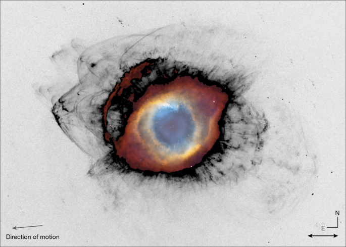
MainThe Helix Nebula (NGC 7293) is one of the closest and brightest planetary nebulae, and therefore a benchmark for resolving how the late-stage ejecta of stars couple to their surroundings. Using the Gaia EDR3/DR3 astrometric solution for the central star (WD 2226-210), we adopt a distance of d = 198.6 (+1.6/−1.8) pc (ref. 10). Imaging of the Helix has shown it to be highly complex. Its bright main nebula comprises an inner disc and a surrounding outer torus, embedded within a larger structure whose upstream side is truncated, consistent with interaction between the expanding asymptotic giant branch (AGB) ejecta and the ambient interstellar medium (ISM)11,12,13. The ionized nebula is threaded by thousands of dense cometary knots and associated molecular material, indicating that much of the ejected material remains in a clumpy, only partially processed phase11,14. Deep imaging and spectroscopy have also revealed a bow-shock feature in the faint outer halo, in the direction of the nebula’s motion through the local ISM12,15. Together, these properties make the Helix uniquely suited to place direct constraints on how fragmented stellar ejecta are dispersed and mixed into the ISM: an essential step in the recycling of mass, dust and newly synthesized elements in galaxies4,9.The Helix Nebula was observed in the light of Hα, [N ii] and [O iii] with the partially built Modular Optical Telephoto Hyperspectral Robotic Array (MOTHRA). MOTHRA is an array of high-end telephoto lenses equipped with tiltable ultra-narrow interference filters, located at the El Sauce Observatory in Chile. Its design evolved from the Dragonfly Spectral Line Mapper at New Mexico Skies Observatory16,17. When completed, MOTHRA will have 1,140 lenses distributed over 30 mounts, and be optically equivalent to a 4.8 m f/0.08 refractor. The data described here are equivalent to roughly 20 minutes of on-source exposure time with the completed array.The MOTHRA Hα image of the Helix is shown in Fig. 1. It shows many features that have not been seen in ionized gas before, such as extensions of the plumes in the northwest and southeast11,13 and turbulent and complex low surface brightness Hα emission in the southwest13. The most striking feature in the Hα image is a forest of arcs and partial arcs on the eastern side of the nebula. We identify at least 22 arcs on the eastern side, labelled 1–22 in Fig. 3 in order of increasing distance from the central white dwarf. Although most of the features appear to be new discoveries, several can be seen in previous GALEX and Hα images. Besides the large and complex feature 14 this includes arcs 3, 10 and 13, among others11,13,15. The arcs are undetected in [O iii] and faint in [N ii]; from the brightest region of arc 14 we measure [N ii]/Hα = 0.06 ± 0.01 and [O iii]/Hα < 0.015 (2σ). We also find faint arc-like features on the western side, at a similar distance from the white dwarf as the much brighter ones in the east.Fig. 1: MOTHRA Hα imaging of the Helix Nebula.The MOTHRA continuum-subtracted Hα image is shown with an inverted grey scale, emphasizing faint outer features. In the bright central regions a combined Hubble Space Telescope and Kitt Peak 4 m image is superposed on the MOTHRA data11. The Hubble Space Telescope image was generated from data in the Advanced Camera for Surveys F502N ([O iii]) and F658N (Hα) filters. The arrow indicates the Gaia-determined direction of motion of the central white dwarf with respect to the ambient gas. The MOTHRA image shows many features at large (roughly greater than 1 pc) distances from the white dwarf that had not been detected in Hα before. The most striking of these are numerous bow shocks on the east side of the nebula, where AGB ejecta encounter the ambient ISM at supersonic relative velocities. Scale bar, 5′ = 0.29 pc. The colour Hubble Space Telescope/Kitt Peak image is reproduced from NASA, ESA, C. R. O’Dell (Vanderbilt University) and M. Meixner, P. McCullough and G. Bacon (Space Telescope Science Institute).Following earlier studies we interpret the eastern features as bow shocks in which expanding stellar ejecta encounter the ISM at supersonic velocities13,15. The velocity of the Helix with respect to the ISM is roughly 36 km s−1 towards 95° east of north in the plane of the sky and roughly 27 km s−1 along the line of sight15,18, for a combined ISM velocity of vISM ≈ 45 km s−1 with respect to the systemic velocity of the nebula. On the eastern side the shock velocity is the sum of vISM and the expansion velocity of the ejecta, vshock, e ≈ |vISM + vexp|. On the western side the ejecta encounter a turbulent postshock wake that has passed through, and mixed with, the planetary nebula, vshock, w ≈ |vwake − vexp|. The wake velocity is expected to be small with respect to the systemic velocity of the nebula. In the case of the well-studied AGB star Mira, the processed gas being shed from the bow shock into the immediate downstream tail lags the star by only roughly 10% (ref. 19); applying the same scaling to the Helix gives vwake = 0−10 km s−1 for the flow on the western side.Using the MAPPINGS V code20 we derive shock velocities on the eastern side of vshock, e = 80−90 km s−1 from the [O ii]/Hα and [N ii]/Hα line ratios (Methods). Subtracting the 45 km s−1 ISM velocity gives an expansion velocity of the ejecta of vexp = 35−45 km s−1, consistent with previously measured Hα kinematics in the region of the brightest bow15. The implied velocity field around the Helix is shown in Fig. 2. Near the east–west axis the shock velocities are roughly 80 km s−1 in the east and roughly 35 km s−1 in the west. For these velocities, shock models predict Hα luminosities that are 1 to 2 orders of magnitude fainter in the west than in the east, consistent with the appearance of the bows on the two sides of the Helix (Methods).Fig. 2: Velocities experienced by fragments.Schematic velocity field around the Helix, for a bulk velocity with respect to the ISM of vISM = 45 km s−1 eastward, a postshock flow velocity of vwake = 5 km s−1 and a radial expansion velocity of the ejecta of vexp = 40 km s−1. The highest velocities are found on the east side, where we see the strong bow shocks.The expansion velocity of vexp = 35–45 km s−1 indicates a dynamical age of the clumps of 20,000–30,000 years at r ≈ 1 pc, predating the formation of the planetary nebula roughly 12,000 years ago21. The material therefore most likely belongs to an older circumstellar envelope that was ejected during the late-AGB phase, and has now fragmented into many individual clumps. This interpretation is strengthened by the fact that the bows lie at approximately the same radius as the roughly 40′ outer WISE 12-μm halo, which has been associated with dust from an AGB wind13. Fast winds and outflows, with velocities that can exceed the canonical roughly 5−20 km s−1 range of the main AGB phase22, are commonly observed during the late-AGB and early post-AGB phases23,24. These flows are often bipolar rather than isotropic25, which may explain why there appears to be a preferred axis connecting the strong bows in the east to northeast of the Helix to the weak bows in the west to southwest.We fit the bow morphologies with a range of functional forms: parabolas, hyperbolas, ellipses and Wilkinoids26. We adopt the parabolic fits as our fiducial model, as they provide a reasonable description of the data and retain the same functional form under projection27. As many of the structures do not show a complete bow, and some are broader and less sharply bounded than ideal thin-shell bow shocks, we do not attach direct dynamical meaning to the adopted fit family itself. Instead, we use the fits to extract geometric quantities (in particular the characteristic curvature scale), and use the variation between fit families as an estimate of the systematic uncertainty. The fitting procedure is detailed in the Methods, with the results shown in Fig. 3. Most of the 22 bows are reasonably well fit by a parabola, although the wings are often closer to hyperbolic27. The brightest bow (14) is more sharply peaked than the model curve; inspection of the region near the apex shows that it is broken up in a complex network of smaller shocks.Fig. 3: Parabolic profile fits to bow shocks.Twenty-two complete and partial bow shocks are identified in the Hα image. They are fitted with parabolas, indicated with the red lines (Methods). Red dots indicate the foci of the parabolas; these correspond to the expected approximate locations of the objects that produce the shocks. The lack of Hα detections near the foci indicates that the objects producing the bows are largely neutral. The bows are numbered according to the distance of the apex to the central star. Two known features, the NE Object and the NE Arc11, are also marked.The foci of the parabolic fits are indicated with red dots in Fig. 3. These are the approximate locations of the shell fragments that produce the shocks, although the exact location depends on the three-dimensional orientation and shape of the bows27. There is generally nothing visible in Hα, [O iii] or [N ii] at or near these locations. The lack of detected emission counterparts at most of the inferred obstacle locations is consistent with the fragments being largely neutral. Our observations thus represent a new observational window on the mixing of AGB and planetary nebula ejecta into the ISM, in which the fragments are identified not by their intrinsic emission but by the shocks that they drive.The nature of the bows changes systematically with distance from the white dwarf: close to the star they are large, thin and well-defined, whereas in the outskirts they are smaller and fuzzier. To quantify this trend without assuming a particular steady-state bow-shock solution, we characterize each structure by the radius of curvature at its apex Rc, as measured from the best-fitting parabola. The relation between Rc and the distance from the white dwarf, r, is shown in Fig. 4. The characteristic size of the bows decreases by two orders of magnitude over the radial range 0.4 pc ≲ r ≲ 1.4 pc. A log-linear fit gives log Rc = 0.34−1.59r, corresponding to an e-folding length of 0.27 pc.Fig. 4: Relation between the size and morphology of bow shocks and their distance from the central star.Left, radius of curvature Rc, determined from fitting parabolas to the bows versus distance from the central white dwarf r. Grey points indicate the location of the apex of the shock and black points indicate the focus: that is, the approximate location of the object that is causing the shock. Yellow numbers identify the bows, ordered by the distance of the apex from the white dwarf. There is a strong dependence, with shocks in the outer parts being smaller. The red line is a fit of the form log Rc = 0.34−1.59r, corresponding to an e-folding length of 0.27 pc. Right, representative morphologies of shocks at a distance r ≈ 0.8 pc from the white dwarf (top) and at r ≈ 1.3 pc (bottom). As r increases, there is an evolution from large, thin, well-defined shocks (4, 6, 7, 8) to small, broad features (16, 18, 20, 22) that we interpret as a sequence of shell fragment disruption.Because Rc is a purely geometric quantity, it does not by itself specify the detailed momentum balance within the flow. It does, however, show that the spatial scale of the coherent bow-forming obstacle decreases strongly with outward distance. This geometric trend is accompanied by a systematic morphological transition: the inner bows are thin and sharply bounded, whereas the outer structures are broader, more irregular, and increasingly clumpy. Taken together, these changes suggest progressive stripping and fragmentation of the dense AGB-shell remnants as they interact with the ambient medium. As material is ablated from the fragments and mixed into the surrounding flow, the surviving dense heads become smaller and more porous, and a larger fraction of the Hα emission probably arises in fragment-associated, mass-loaded mixed gas rather than in a geometrically thin, well-defined forward shock8,28,29.In this interpretation, the bows are both signposts of the fragments and agents of their destruction. The shocks are powered by the relative kinetic energy of the fragments and the ambient flow, and their presence implies ongoing momentum transfer, ablation and mixing8,28. Interpreting the radial locations of the bows, ri, as a time sequence for outward evolution, ti ≈ ri/vexp, the slope of the Rc–r relation implies a characteristic timescale for the loss of coherent bow structure. For the expansion velocity derived from the shock velocities in the east, vexp ≈ 40 km s−1, the curvature scale declines with an e-folding time τRc ≈ 7 × 103 years. We therefore infer that the bow-forming AGB-shell fragments are disrupted on a timescale of order 104 years. This estimate should be interpreted as the survival time of the coherent dense fragment–bow system, rather than as a direct measurement of a specific momentum or mass-loss rate.Classical AGB–ISM bow shocks such as Mira trace a single, wind-driven stand-off interaction centred on the mass-losing star6, and far-infrared surveys show that such global wind–ISM interaction structures are common around evolved stars7. However, these long-lived6 (roughly 105 years) large-scale bows primarily map where the wind meets the ISM; they do not directly constrain how fragmented ejecta are ultimately assimilated. In the Helix outer halo we instead resolve numerous compact bow shocks with no luminous source at their foci, indicating that the AGB–ISM interaction has fragmented into dense, line-dark obstacles that are progressively ablated and entrained. The roughly 104 years characteristic disruption time for the fragments can therefore be interpreted as the relevant timescale for recycling of late-AGB ejecta into the ISM.More broadly, stellar mass loss is a major channel by which galaxies recycle gas, metals and dust back into the ISM30, yet the efficiency and duration of the final, fragment-driven AGB–ISM assimilation step remain poorly constrained observationally6,31. Galaxy formation simulations therefore rely on subgrid turbulent mixing and diffusion prescriptions to represent unresolved transport32,33,34. Our empirically inferred roughly 104 years disruption time implies that once AGB ejecta are fragmented and exposed to the diffuse medium they lose their coherent identity rapidly, providing a benchmark for models of recycling and feedback.Our conclusions can be tested and extended in several ways. The Helix is a fairly typical planetary nebula, and we should see similar fragment-driven bow shocks in the outskirts of other planetary nebulae. Because of the steep relation between Hα luminosity and shock velocity such features will be most readily detected when the bulk motion of the nebula with respect to the ISM exceeds roughly 40 km s−1. When more examples are found, it will be interesting to see if the mixing timescale depends on the shock velocities. Such observations will be within easy reach of the completed MOTHRA. Furthermore, by analogy with the molecular cometary knots in the Helix14,35,36,37, the Hα-dark clumps whose presence is inferred from the shocks could be detectable in CO rotational lines and, particularly, in the H2 1–0 S(1) 2.12-μm line.MethodsObservationsThe Helix Nebula was observed as a commissioning target during the early construction phase of MOTHRA. When completed, the array will comprise 1,140 Canon 400 mm, f/2.8, II/III telephoto lenses distributed over 28 narrow-band mounts and 2 broadband mounts. Each narrow-band mount has 38 lenses: 18 are equipped with an Hα filter, 8 with [O iii] λ5007, 8 with [N ii] λ6583 and 4 are continuum filters. The widths of the ultra-narrow interference filters are 0.71 nm for [O iii] and 0.93 nm for Hα and [N ii], corresponding to a velocity bandwidth of roughly 430 km s−1. The continuum filters, two for Hα and [N ii] and two for [O iii], are roughly 90 nm wide with a roughly 33-nm notch in the middle at the location of the emission lines. These filters therefore measure the continuum at the wavelengths of the lines, without being contaminated by them.The observations reported here were obtained on 16 November and 19–24 November 2025, when the first five mounts of MOTHRA were operational. As the number of active lenses varied during the observations, we express the exposure time as single-lens equivalent hours, that is, the exposure time multiplied by the number of lenses that were in use during the observation. In Hα the on-target exposure time was 172.5 single-lens equivalent hours, corresponding to 20 min with the 504 Hα lenses that the completed MOTHRA will have.Data reductionThe data reduction includes several steps that are unique to the design of MOTHRA and its prototype, the Dragonfly Spectral Line Mapper16,17. The roughly 400 km s−1 wide interference filters are placed in front of the lenses, and specific wavelengths are chosen by tilting the filters. Owing to the large (roughly 3°) field of view, the wavelength of the bandpass is not constant over the image but varies as a function of the angular displacement of the target relative to the projected tilt axis of the filter, as well as the angular distance to the optical axis. As a result, the sky background is complex: sky emission lines appear as broadbands in the image, particularly at the large tilts that are used for Galactic objects16. For the Helix observations, we obtained offset sky exposures in a circular pattern around the science field to model the background. Bracketing sky exposures were combined and subtracted from each individual science frame, before combining the science data.A colour image of the Helix is shown in Extended Data Fig. 1, created from the [O iii], Hα and [N ii] data. It is well established from narrow-band imaging and line-ratio mapping that the morphology of planetary nebulae varies strongly between different emission lines, with low-ionization structures often enhanced in [N ii] relative to [O iii]38,39,40. The Helix shows the same behaviour in its central regions and faint outer halo11,21,41. In the MOTHRA images, the forest of bow shocks is relatively bright in Hα and is faint in [O iii] and [N ii].The final step in the data reduction is the subtraction of continuum emission from the narrow-band data; this was done by matching the point spread functions of the two images and scaling the continuum image to match the normalization of the narrow-band image. Remaining residuals were filled in with the maskfill code42. The depth of the images was determined with the sbcontrast method, which empirically determines the contrast sensitivity on a desired spatial scale43. The reduced and sky-subtracted narrow-band images reached a 1σ depth of roughly 2 × 10−19 erg s−1 cm−2 in Hα on 1′ scales.Shock velocityTo interpret the observed emission-line ratios we computed a grid of radiative shock models using the MAPPINGS V code20. The models were run with Solar abundances and included a self-consistent treatment of the photoionizing precursor, in which the upstream ionization and temperature structure were iteratively determined from the radiation field produced in the postshock cooling zone. We adopted a preshock hydrogen density of nH = 5 cm−3, consistent with the fiducial density used in recent MAPPINGS V benchmark calculations44, and appropriate for diffuse circumstellar and interstellar environments. The results were insensitive to the choice of nH, as the lines formed when much higher densities were reached. The magnetic field strength was parameterized through α ≡ B/√nH (with B in μG and nH in cm−3), which controls the degree to which magnetic pressure limits compression in the postshock cooling zone20.We explored two representative regimes: a weak-field case with α = 1, which effectively captured the hydrodynamic limit (the results were virtually identical for all values α ≲ 1), and a magnetically supported case with α = 2, for which magnetic pressure significantly reduced the maximum compression. Shock velocities were sampled finely in the range vshock = 20−115 km s−1 to resolve the transition in ionization structure associated with the onset of [N ii] and [O iii] emission.The results are shown in Extended Data Fig. 2. The line ratios are a strong function of shock velocity in this regime: the postshock temperature increased as T ∝ vshock (ref. 2), leading to a rapidly increasing flux of ionizing photons from the cooling zone and its associated precursor20. For [O iii], the onset was abrupt once the radiation field became sufficiently hard to sustain an extended O++ zone, whereas lower-ionization species such as [N ii] responded more gradually. The observed upper limit on [O iii]/Hα and measured [N ii]/Hα (the grey bands in Extended Data Fig. 2) indicated a shock velocity of vshock = 80−90 km s−1 depending on the magnetic field strength, and we use vshock = 85 ± 5 km s−1 in the main text.Hα luminosity as a function of shock velocityThere is a clear asymmetry in the brightness of shocks in the outer Helix Nebula, with all strong shocks located on the eastern side. As can be seen in Fig. 1 and Extended Data Fig. 1, there seems to be a corresponding region on the other side of the nebula, showing rounded arcs and bubbles that are only detected in Hα. In Extended Data Fig. 3 we show a side by side comparison of the two regions. Here we ask whether the difference in brightness between the eastern and western shocks can be explained by the difference of the shock velocities.The right panel of Extended Data Fig. 3 shows the Hα luminosity as a function of shock velocity, from the MAPPINGS V code20. At low velocities, the Hα luminosity rises steeply with shock velocity as the shock progressively ionizes neutral hydrogen. At higher velocities, once the radiative precursor pre-ionizes the upstream gas, the hydrogen ionization fraction approaches unity and the Hα emissivity no longer tracks the mechanical energy flux. Instead, additional energy is channelled into heating and metal-line cooling, resulting in a flattening of the Hα–velocity relation.Grey bands show the inferred shock velocities, 85 ± 5 km s−1 on the east side and 35 ± 10 km s−1 on the west side (main text). Because of the steep rise of the Hα–vshock relation in this regime, the Hα luminosity is expected to be 1 to 2 orders of magnitude higher on the east side than on the west side. The difference in the observed surface brightness is a factor of roughly ten, broadly consistent with the shock models.We note that the Hα features on the west side are probably not related to the high velocity jet in that region, even though they appear to be in front of it in projection (Extended Data Fig. 3). The jet has a velocity of roughly 300 km s−1, measured directly from Hα and [N ii] spectroscopy15, and if the shocks were driven by the jet they would show strong [O iii] emission.Fitting of bow shocksThe bows are fit in the following way. A bow is initially characterized by five manually selected (x,y) positions: two marking the end points of the visible arc, one marking the approximate apex and two points in between the end points and the apex. Next, a second-order polynomial is fit to these five points. This fit provides a reasonable approximation of the area of the image where the bow is located. A band of typical width ±20 pixels is defined around the polynomial fit. Within this band the ridge of the bow is identified by determining the local maximum in bins along the polynomial. To enhance contrast, an unsharp-masked version of the Hα image is used to measure the ridge.With the ridge line measurements in place, a fit to an analytic function is performed. Following earlier work27, we fit four families of functions: parabolas, hyperbolas, ellipses and Wilkinoids26. For each functional form we determine the associated radius of curvature Rc and the related distance between the apex and the object Ro. For a parabola Ro = Rc/2; for a hyperbola and an ellipse Ro = Rc/(1 + e), with e the ellipticity and for a Wilkin profile Ro = 3Rc/5. The five manually selected points are not used in the fit. After the initial fit the band is redefined, now on the basis of the specific analytic function rather than the polynomial, and the ridge line measurements and fit are repeated. The process is illustrated for eight of the bows in Extended Data Fig. 4. The fits are stable for the 22 bows that we identify in the image.As discussed in the main text, we use the parabola as the fiducial profile, and take the root mean-square ranges in Rc and Ro from the four fits as uncertainties.