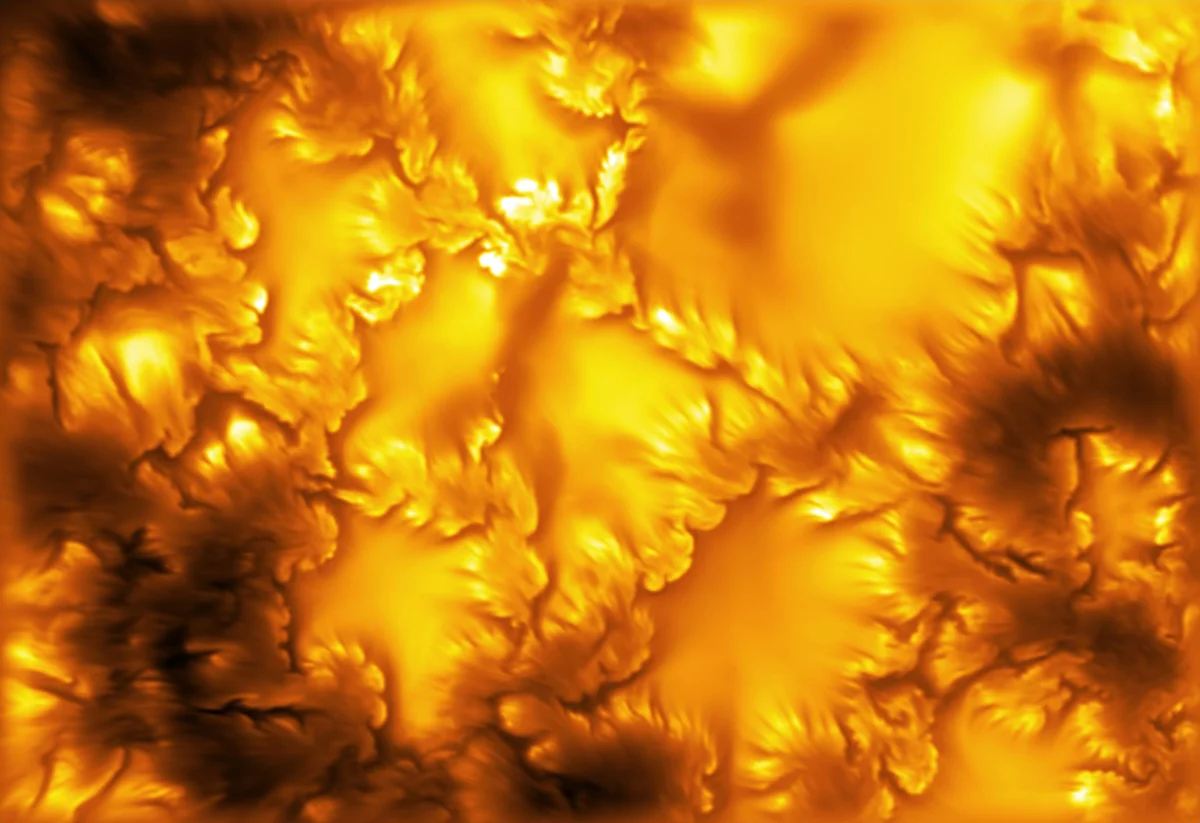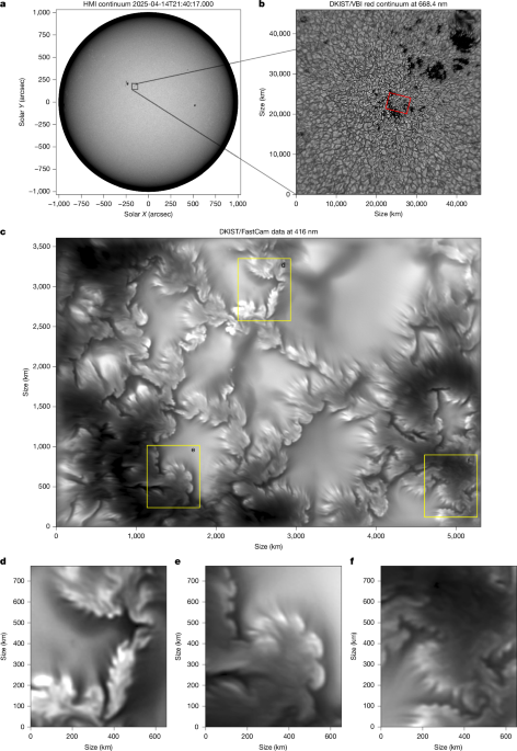
MainSince their original formulation by Lord Kelvin3 and Hermann von Helmholtz4, Kelvin–Helmholtz instabilities (KHIs) have been observed and investigated across many areas of physics, including fluid dynamics5, oceanography6, heliospheric environments such as planetary magnetospheres7,8,9,10 (for example, Earth, Mars, Venus, Mercury, Jupiter and Saturn) and other astrophysical systems11,12,13,14,15. In the solar atmosphere, KHIs have long been the subject of both theoretical and observational studies1,2,16,17,18,19,20. Corrugated boundaries observed in coronal mass ejections are often interpreted as possible signatures of this instability16,17,18.Solar and stellar magneto-convection produce complex plasma flows in the photosphere that evolve from coherent laminar motions into small-scale, unstable structures. Theoretical studies indicate that these flows in the solar photosphere can generate velocity shear layers around magnetic flux concentrations (MFCs) and trigger the KHI1,2. The existence of KHIs in the Sun’s photospheric layers has not been observed in the past, probably because the characteristic spatial scale is not easily accessible by telescopes with aperture sizes below 2 m.The observations made by the Daniel K. Inouye Solar Telescope (DKIST)21 at a wavelength of 416 nm reported here are of a magnetically active region in the vicinity of a sunspot (Fig. 1). At this wavelength, the visible solar surface is dominated by convective motions (granules) interlaced with small-scale MFCs (Fig. 1). This scene contains several larger coherent structures (pores). The interfaces between the magnetic features and the granulation in these images display a structure very different from the relatively smooth, blurry interfaces typically seen in lower resolution images. DKIST reveals these interfaces to be composed almost entirely of vortex-like structures and striations, drastically changing the solar scene compared with previous observations. Fig. 1: A view of the solar photosphere at a spatial resolution of 19 km.a, A contextual SDO/HMI continuum full-Sun image from 14 April 2025. The black box marks the part of the active region (NOAA 14060) observed with DKIST/VBI. b, Zoomed-in view of the boxed area in a at 21:40:40 ut. A subfield outlined by the red box indicates the FastCam FoV. The dark areas are pores, where—like the larger sunspots—the strong magnetic field inhibits convective energy transport outwards towards the solar surface, thereby creating a cooler plasma environment. c, The photosphere captured with DKIST/ FastCam at 21:39:15 ut in the blue continuum (416 nm) at a resolution of approximately 19 km. d–f, The zoomed-in subregions outlined with yellow boxes in c show prominent KHI examples.The image time sequence reveals the ubiquitous formation and evolution of vortices at the interface of magnetic elements, with the smallest vortices being near the theoretical diffraction limit of DKIST of approximately 19 km on the Sun at this wavelength (Fig. 1c–f, Extended Data Fig. 1 and Supplementary Video 1). In Extended Data Fig. 2 we show the result of an analysis of 47 vortices in the observed field. The histogram demonstrates that the characteristic spatial wavelength—the spatial distance between vortices—was 65 km, with sizes ranging from 25 km to 170 km. The growth rate \({\gamma }_{\mathrm{im}}\), defined as the exponential factor by which the deformation of the magnetic interface (boundary) increases over time (Methods), has values between 0.014 s−1 and 0.054 s−1 for prominent examples in the field of view (FoV) (Extended Data Table 1). We estimated these growth rates by tracking boundary perturbations of the unstable interface where vortices form (Extended Data Fig. 3). The measured apparent velocities (the horizontal propagation speed of vortices around the magnetic elements) ranged between 0.67 km s−1 and 3.0 km s−1 (Extended Data Table 1).We compared the observed structures with numerical radiation magnetohydrodynamics (MHD) simulations of the solar atmosphere carried out with the MURaM22 code. The simulations model a plage region with a net flux, starting from an initially vertical field equivalent to that of the observed scene (Methods and Supplementary Fig. 1) and were computed for a spatial discretization size of 3.2 km, yielding a resolution comparable with that of DKIST. With these spatial discretization sizes and magnetic field strengths, the numerical simulations show structures like those in the observations (Fig. 2 and Extended Data Fig. 4). The prominent shape of the vortices seen in both the observational and synthetic data matches the morphological structure of the KHI (Figs. 1–3). Based on the evidence presented so far and on that presented below, we will refer to the vortices and striations as KHI structures.Fig. 2: Overview of the MURaM simulation.a, Vertical magnetic flux density at the height where the average optical depth τ500 is unity near the interface between magnetic and non-magnetic regions. b, Horizontal velocity field at the same height. c, Synthetic emergent intensity at 500 nm at disk centre computed from the MURaM cube. d–f, Zoomed-in images of the regions indicated by the yellow boxes in the top panels: vertical magnetic flux density (d), horizontal velocity field (e) and synthetic emergent intensity (f). The arrows in e indicate the direction of the plasma flows.Fig. 3: Observed versus synthetic KHI vortices.a–c, Evolution of KHI vortices in the observed (a) and synthetic (b) intensities and in the line-of-sight magnetic field (c) in MURaM at the height where the average \({\tau }_{500}=1\). The synthetic intensities were computed at disk centre at a wavelength of 500 nm. The four leftmost images are snapshots at four times (the simulations could follow the scene for a longer time). The rightmost panels are time–distance diagrams produced along the cyan dotted lines, displaying the dynamics of the KHI vortices. In these panels, the observed and synthetic data cover exactly the same spatial and temporal ranges so that they can be compared one to one. T–D diagram, time–distance diagram.The simulations show an important ingredient not measured by the observations, the horizontal plasma velocity. It runs parallel to the sharp interface of the strong magnetic field and displays a strong gradient there, thereby creating the optimal environment for the onset of KHI (Fig. 2b–e).Magnetic fields can have a stabilizing influence on the KHI: the component parallel to the shear flow tends to suppress the instability, whereas the perpendicular component provides no stabilization23. Strong fields dominating the observed and simulated plage regions are nearly vertical at the solar surface and, hence, mainly perpendicular to the horizontal shear flow. Linear theory predicts that instability growth is maximized when the Kelvin–Helmholtz wavevector is aligned with the flow direction23, consistent with our observations and simulations showing that the KHI develops ubiquitously along horizontal shear layers surrounding vertically oriented MFCs. Figure 2 and Supplementary Videos 2–4 illustrate how laminar granular flows, the fundamental convective pattern of the photosphere, converge towards MFCs and form strong horizontal shear layers that trigger the KHI: because the parallel components of the flow are weakly coupled across the interface to magnetic regions, a strong shear can develop along the interface.We investigated the instability parameters in the MURaM simulations by employing the same techniques used on the observed images. We synthesized spectra covering the wavelength range 415.32 nm to 416.7 nm at a heliocentric angle of approximately 14°, corresponding to a viewing angle μ of \({\mu }=\cos (14^\circ )\approx 0.97\), to match that of the observed FoV on the Sun (Extended Data Fig. 4). Synthetic filtergrams were generated using the band-pass characteristics of the interference filter employed during the observations (Extended Data Fig. 4). The resulting synthetic images were spatially low-pass filtered to match the DKIST spatial resolution because the image reconstruction algorithm for the observed data already removes the optical transfer function of the telescope as part of the reconstruction process. The results are presented in Extended Data Fig. 5 for 94 instability occurrences. The histogram peaked at a characteristic instability wavelength of 49 km. An evaluation of the growth rate for several notable examples in the synthetic images yielded values in the range 0.027 s−1 to 0.059 s−1 (Extended Data Table 1). The instability wavelength and growth rate in the synthetic images are comparable with those measured in the observations, as are the measured apparent vortex velocities, which ranged from 1.6 km s−1 to 2.8 km s−1 (Extended Data Table 1). The consistency between the numerical simulations and observations demonstrates that the numerical model sufficiently captures the physical processes leading to the KHI.The measured intensity in the filtergrams primarily originated from atmospheric layers near the \({\tau }_{500}=1\) surface (hereafter, \(\tau =1\), unless otherwise indicated), where \({\tau }_{500}\) is the optical depth at 500 nm (Methods). This layer defines the base of the photosphere, and vertical heights are measured relative to it. Because the \(\tau =1\) surface corresponds to a corrugated sheet that varies in geometrical height depending on, for example, the level of magnetization of the emitting plasma, we use its mean height, averaged over the FoV of the simulation, as our reference (z = 0 km). The intensity signature of the vortices compares well with that of the magnetic field morphology at z = 0 km (Supplementary Fig. 2).For a finite-width shear layer, such as the hyperbolic tangent velocity profiles presented in our simulations, the KHI wavelength of the fastest-growing mode scales with shear layer thickness23. In the linear regime, the shear layer thickness is related to the expected KHI wavelength through equation (2), which in turn is related to the instability growth rate and phase speed23. Extended Data Fig. 6 shows the solutions of equation (2), computed using the parameters (shear layer thickness, shear velocity and density contrast) derived from the simulation for the five cases listed in Extended Data Table 1. The results demonstrate that the growth rates and phase speeds estimated directly from the data are consistent with the predictions of the linear KHI theory23, in which the plasma flow becomes unstable perpendicular to the magnetic field.Measurements of the velocity shear layer thickness from the numerical simulations yield values of approximately 12 km (Extended Data Table 1, Extended Data Fig. 7 and Supplementary Figs. 3–6). Ignoring the weak dependencies of the KHI spatial wavelength on density and average shear velocity, linear theory23 predicts that the most unstable mode has spatial wavelengths between 60 km and 100 km (Extended Data Fig. 6), close to the measured observation values.The KHI structures rapidly enter the nonlinear regime. They exhibit fully developed vortices along with rapid vortex merging and the formation of secondary, smaller-scale KHIs on the larger vortices (Extended Data Fig. 8). This shows that the KHI makes a critical contribution to the development of turbulence in these boundary layers. The KHIs analysed in this study can be considered as a source of turbulent diffusivity24, with a value of ηtur ≈ 1/3uλ, where u is the typical turbulent velocity and λ is the typical length scale of the flow. The scale λ ≈ 65 km of the KHI wavelength and average shear velocity u ≈ 3 km s−1 yield an estimated turbulent diffusivity 0.65 × 1012 cm2 s−1 in strong magnetic field regions (stronger than equipartition), where turbulence is normally suppressed. This diffusivity leads to a mixing between magnetized and mostly unmagnetized plasma and allows low-entropy material present at the edge of granules to enter the magnetized plasma, thereby affecting the properties of downflows and convective energy transport beneath the solar surface.In the MURaM simulations, KHI vortices develop in the horizontal planes over a vertical depth range \(z\in \sim [100,-400]\) km. They maintain the same phase and wavelength across all heights, so that they are best described by vertically extending rolls (Fig. 4 and Extended Data Fig. 9). The amplitude and, hence, the growth rate of the perturbations increase towards the deeper layers (below \(z < 0\) km) (Extended Data Fig. 9). This amplification occurs because magnetic stabilization is weaker in the deeper layers where the magnetic field is more vertically oriented. The plasma beta (ratio of gas to magnetic pressure) is higher due to the higher plasma density (Supplementary Fig. 7), which allows the velocity shear to drive the instability more efficiently. Therefore, in the deeper layers, the KHI at the magnetic boundaries leads to fragmentation, and it splits the monolithic magnetic elements into several smaller structures (Fig. 4 and Supplementary Video 5). This magnetic stratification (a single magnetic element at the visible solar surface that connects to several strands below it) resembles the picture proposed by Parker25 for much larger magnetic features, sunspots, there albeit in response to a fluting instability rather than a KHI25,26.Fig. 4: Temporal evolution of the KHI in the MURaM simulation, rendered with the VAPOR code37.a, Three-dimensional structure of the vertical magnetic field at t = 0 s and t = 174 s, demonstrating the impact of the developing KHI on the magnetized plasma. The height coordinate is relative to the \(\tau =1\) surface. b, A horizontal cut at the \(\tau =1\) surface for three time steps illustrating different phases of KHI development. c, The same for the layer approximately 370 km below the \(\tau =1\) surface. The signature of KHI vortices and their evolution within the horizontal velocity field (black arrows) is clearly visible (Supplementary Video 5).Observed and synthetic photospheric maps show fine-scale dark striations rooted in the KHI vortices and extending outwards (Figs. 1–3). Supplementary Videos 1–4 illustrate that the KHI vortices and their associated striations exhibit coherent dynamics. The morphological and dynamical properties of the striations in the observed and synthetic filtergrams are in notable agreement (Fig. 3 and Supplementary Fig. 8). Photospheric striations at the boundaries of magnetic elements have been detected previously using high-resolution observations27,28,29,30. Striations seen in filtergrams are associated with spatial and temporal modulations of the photospheric magnetic field, which produce corresponding variations in density and opacity along the line of sight31. Despite recent large advances30, the physical origin of the magnetic field variations responsible for the formation of the striations has not been established in either observations or simulations. Using DKIST data together with numerical simulations, we demonstrate that these variations arise from the KHI, which corrugates the boundaries of the MFCs. Similar magnetically induced striations are observed in more distant astrophysical environments, such as molecular clouds like the Polaris flare32 and Taurus clouds33, where the KHI may play a role in creating striated structures.Magnetic structures, such as spicules, prominences and coronal loops, that create the fabric of the outer solar atmosphere are rooted in photospheric MFCs. Changes in the topology of the photospheric magnetic field should influence the structure of the entire solar atmosphere. The KHI, by continuously distorting and perturbing magnetic elements, can excite MHD waves and dissipate energy through vortices that can subsequently break down into turbulence. The nonlinear evolution of the KHI at the boundaries of MFCs in the MURaM simulation shows numerous examples of small-scale vortices forming on top of larger vortices, which may represent a forward turbulent cascade (Extended Data Fig. 8). In other cases, as the KHI amplitude grows, vortices merge and evolve into a more turbulent state, indicative of an inverse cascade.Footpoint motions of the magnetic structures in the solar photosphere are the primary source of free magnetic energy, which in turn powers most solar activity, including energetic brightenings from nano-flares to flares, jets and coronal mass ejections. The same energy reservoir is also thought to power the enigmatic heating of solar and stellar coronae34. A central theoretical concept for generating free magnetic energy is magnetic flux braiding35, which creates non-equilibrium magnetic configurations through the interlacing of field lines. Such systems dissipate energy through electric current sheets and magnetic reconnection while relaxing towards a lower energy state36. The physical drivers of braiding motions remain poorly constrained observationally. The observed vortices generated by KHI could provide an efficient source of small-scale, omnipresent magnetic flux braiding.MethodsObservations and data reductionIn this work we present observations acquired on 14 April 2025 between 21:38 ut and 21:41 ut using the world’s largest telescope for optical and infrared observations of the Sun, DKIST21. During the data acquisition, the atmospheric conditions were variable, with Fried parameter values during the best periods measured around \({r}_{0}\approx 12\,\mathrm{cm}\). The DKIST wavefront correction system was operating in diffraction-limited mode at the time of the observations, as it was measuring and correcting all optical modes that it is capable of detecting. In this work, we focus on the first target of the day, a region containing pores near an active region (NOAA 14060) close to the disk centre with helioprojective Cartesian coordinates (X = −162 arcsec, Y = 168 arcsec), corresponding to \(\mu \approx 0.97\) (Fig. 1).A dataset was acquired with a diagnostic (FastCam) set-up at DKIST, which was built as a collaborative effort between the National Solar Observatory and the Max Planck Institute for Solar System Research. The set-up was installed in front of the spectrograph entry slit of the visible spectro-polarimeter and removed at the end of the data acquisition for the diagnostic test. The optical set-up enhanced the operation of the feed telescope of the visible spectro-polarimeter, which did not have any other powered optics, resulting—with the pixel cell size of 5.5 μm for the Max Planck Institute camera—in a pixel size of ∆s ≈ 0.00825 arcsec px−1, corresponding to approximately 6 km px−1 on the solar surface. The wavelength chosen for the observation was 416 nm, and we used a narrow band-pass with a full-width at half-maximum of 0.5 nm. The region of interest read out by the camera was set to 2K × 1K px2, which meant that the sensor could be read out at a rate of 740 frames per second while maintaining an exposure time of 100 μs. The camera was equipped with a phase-diversity beam-splitter assembly, which imaged two fields, one in-focus and the other with a de-focus of approximately 0.4 waves root mean square. The two fields were imaged side-by-side onto the sensor in a phase-diversity set-up38,39, which allowed us to determine the residual wavefront aberrations that remained after the correction by the adaptive optics system40. The solar FoV visible in both the focused and the de-focused images corresponds to approximately 5,800 × 4,350 km2 on the Sun (8 × 6 arcsec2). The time span covered by the dataset analysed in this work is about 3 min. The frames observed with this camera were image-reconstructed using multi-frame blind deconvolution41, a technique that can be used to numerically model and remove residual atmospheric aberrations from the data. The algorithm used 2,000 dark- and gain-calibrated camera frames to compute one reconstructed science frame. After image reconstruction, the effective cadence of the imaging data was 2.7 s. We estimated that most frames achieved a spatial resolution of 19 km, the Rayleigh diffraction limit at 416 nm, as inferred from the full-width at half-maximum of the finest structures in the data.Context imaging was provided by the visible broadband imager (VBI)42, an imaging instrument capable of acquiring large-FoV short-exposure data sequences at a single wavelength within 3 s. In this experiment, the VBI was configured to acquire sequences of 80 frames alternating in wavelength between the red continuum (668.4 nm) and the Hα line (656.3 nm; not shown), with sampling in the images corresponding to 12.3 km px−1 (0.017 arcsec px−1). The frames of each consecutive sequence were image-reconstructed using speckle reconstruction algorithms43 to remove residual seeing effects over the large FoV of approximately 50 × 50 Mm2 (69 × 69 arcsec2). Even though the VBI red channel was started with a 3-min delay with respect to the FastCam data that are presented here, the FoV clearly still contains the (evolved) structure of the higher spatial resolution dataset (Fig. 1).Full disk observations were provided by the helioseismic and magnetic imager onboard the Solar Dynamics Observatory (SDO/HMI)44. Figure 1a shows a photospheric continuum image from the HMI at 21:40 ut. The HMI image was coaligned with DKIST/VBI/FastCam data using the SolarSoft auto_align_images function through a cross-correlation (Fig. 1).Numerical simulations and spectral synthesisHere we compare the observations with MHD simulations performed with the MURaM code22. So that we could perform the simulations at a very high spatial resolution, we focused on a small domain of extent 6.144 × 6.144 × 2.048 Mm3 (with the third dimension, z, being vertical), which is comparable with the high-resolution FastCam FoV. In the vertical direction, the domain extended approximately 1.367 Mm below z = 0 Mm and 0.681 Mm into the overlying atmosphere. A solar-like configuration with granulation driven by radiative losses could not be achieved in the numerical simulation without the overlying stable atmosphere. A realistic photosphere was essential for making the connection between numerical models and observations. We started from a relaxed hydrodynamic simulation to which we added the vertical magnetic field component extracted from the corresponding HMI magnetogram for the observed region (Supplementary Fig. 1). We initialized the domain with a strictly vertical magnetic field of the form \(n{B}_{z}-(n-1)\langle {B}_{z}\rangle \), where \({B}_{z}\) was taken from an HMI magnetogram and was enhanced to compensate for the field dispersal that occurred due to granular motions when the simulation was further relaxed for about 1.8 h (n is the enhancement factor). After the relaxation, the individual flux concentrations were no longer impacted by the initial state. To achieve a realistic simulation of magneto-convection, the critical parameter is the net flux imbalance, which was unchanged by the enhancement. Therefore, the enhanced HMI magnetogram was used solely to create a set-up that looks more closely like the observed distribution, and it was not needed for the development and study of KHIs. We found that a choice of \(n=2.5\) led to a large-scale magnetic field distribution comparable with the HMI magnetogram and the formation of pores that resemble those observed (Supplementary Fig. 1). After initialization with the enhanced magnetogram, the simulation ran for 4,980 s with 12.8-km grid spacing, followed by 1,200 s with 6.4 km and then another 1,200 s with 3.2-km grid spacing. The sequence we analysed also covers 480–720 s in the 3.2-km sequence or 5,460–5,700 s since the initialization with the HMI magnetogram. The simulation was computed with 12 opacity bins and used the Asplund 2009 opacities45.The grid scale of 3.2 km was greater than the diffusive length scale expected in the photosphere of approximately 1.4 km based on a Spitzer diffusivity \(\eta \) = 2 × 108 cm2 s−1 (ref. 46) and a timescale \(\tau \) = 100 s using \(l\approx \sqrt{\eta \tau }\). The use of the numerical diffusivity22 is, thus, justified for the simulations presented here. However, a spatially dependent Spitzer diffusivity would need to be used for higher resolution simulations.Developed snapshots of the simulation were used to generate the synthetic spectrum for a wavelength interval between 415.32 nm and 416.7 nm, using 500 spectral points with the one-dimensional version of the Rybicki–Hummer radiative transfer code47 in local thermodynamic equilibrium (Extended Data Fig. 4c). The syntheses included molecular (CH and CN) and atomic lines and the continuum within the band-pass. Intensities were also synthesized at a single continuum wavelength of 500 nm. To save computational time, the vertical grid space was reduced to 9.6 km by using only every third grid point along the vertical axes. We synthesized spectra at disk centre and towards the solar limb at \(\mu =1\) and \(\mu =0.97\), respectively. To synthesize 416 nm intensities at \(\mu =0.97\), the MURaM cube was modified by shifting each horizontal layer relative to the layer below by \(\Delta z\,\tan (\theta )\), where \(\Delta z\) represents the vertical grid spacing and θ is the heliocentric angle, defined as the angle between the line of sight and the solar surface normal. This adjustment aligned the slanted line-of-sight direction vertically. Pixel sampling was foreshortened along the y direction by a factor of \(\mu \) and increased along the z direction by a factor of \(1/\mu \) for the \(\mu =0.97\) data. To closely replicate the DKIST 416-nm filtergrams, the synthetic data were multiplied by the transmission profile of the interference filter employed in the diagnostic set-up (Extended Data Fig. 4c) and integrated over the wavelength range covered by the filter.Extended Data Fig. 4a,b demonstrates that all common features observed in the 416-nm filtergrams were reproduced in the synthetic images, including KHI vortices and striations. Extended Data Fig. 4c shows the synthetic spectrum averaged over the full FoV of the simulation, overplotted with a solar atlas48 with the same wavelength range as observed by a Fourier transform spectrometer. The two spectra agree to a high level of detail, demonstrating that the simulation accurately reproduced the observed spectral features. The close agreement between the synthetic and observed spectra and images confirms that the simulated data serve as a powerful diagnostic tool for interpreting 416-nm intensity observations.From the MURaM snapshot, we calculated the height of the surface where the optical depth reached unity at different wavelength positions along the synthesized spectral interval (Extended Data Fig. 9k,l). Extended Data Fig. 9l shows that the heights of \(\tau =1\) and \({\tau }_{415.91}=1\) (as well as other 416-nm continuum wavelengths) are very similar with only marginal differences, indicating that these two continuum wavebands formed at nearly the same geometrical heights. We used the optical depth at 500 nm to select the heights at which KHI parameters were directly studied in the MURaM cube and compared with the synthetic 416-nm filtergrams.Historically, striations have been observed and studied primarily at inclined viewing angles27,28,29,30. Our simulations show that they are also present in the disk centre. Extended Data Fig. 9k confirms that the structures seen in the disk-centre filtergrams arose from opacity variations. Their appearance in the emergent intensity is closely correlated with spatial variations in \({B}_{z}\) and anticorrelated with density in the layers above the KHI formation heights (Supplementary Fig. 9). These variations shift the geometrical height at which the emergent intensity forms, giving rise to the appearance of striations in the disk-centre synthetic filtergrams. This is the same physical mechanism that produces striations at inclined viewing angles28,29,30,31. An inclined viewing geometry makes these features appear longer and more extended towards the limb and, therefore, easier to detect. Our results, however, indicate that they should also be observable at disk centre, given a sufficiently high spatial resolution.KHI growth rate in linear MHD theoryThe linear theory of the KHI in MHD systems shows that the instability grows fastest when the shear flow is perpendicular to the magnetic field and the wavevector is aligned with the shear velocity23. For finite and continuous velocity profiles, the fastest-growing wavelengths are determined by the thickness of the velocity shear layer.Chandrasekhar23 investigated the KHI in a slab geometry consisting of two adjacent incompressible fluids with different densities separated by a finite-width shear layer of intermediate density in which the velocity varies linearly from −\({U}_{0}\) to +\({U}_{0}\) across the layer. Specifically, the velocity and density profiles are given by equation (1) (Supplementary Fig. 10):$$\begin{array}{lll}x < -d/2, & {\rho }_{1}={\rho }_{0}(1+{\epsilon }), & U=-{U}_{0},\\ -d/2 < x < d/2, & \rho ={\rho }_{0}, & U=2{U}_{0}x/d,\\ x > d/2, & {\rho }_{2}={\rho }_{0}(1-{\epsilon }), & U={U}_{0}.\end{array}$$
Ubiquitous Kelvin–Helmholtz instabilities driving plasma mixing on the Sun - Nature
High-spatial-resolution observations of the solar photosphere reveal a far more complex and dynamic solar scene than previously observed and show that ubiquitous Kelvin–Helmholtz instabilities drive plasma mixing on the Sun.
8,454 words~38 min read