SummaryWith Dedicated Model Inference on the Together AI platform you can get your deployments to autoscale on metrics the inference engine actually understands, such as in-flight requests, TTFT, GPU utilization, token throughput. You can set replica bounds, pick a metric and target, and then tune two windows that control how eagerly it scales up and how patiently it scales down. Understanding and choosing the right metric is important because it determines how your deployment will behave under peaky traffic and impacts the latency your users will see. Below we'll cover how to choose the right metric to autoscale on and show an experiment where the same load was replayed under three different autoscale policies.Over- and under-provisioning are both expensiveWith dedicated inference you pay per replica-minute, which makes capacity planning a balance between two failure modes:Over-provision - you're paying for GPUs to sit at 15% utilization just so that you can handle the peak traffic when/if it arrives. Almost never viable, especially in the current GPU constrained environment.Under-provision - your p95 degrades sharply the moment traffic exceeds what your replicas can batch. LLM serving degrades nonlinearly: a replica at its concurrency limit doesn't get "a bit slower," it starts queueing, and TTFT can blow up from 200ms to 15s."Just autoscale it" is the obvious answer, and for stateless web services it mostly works. But LLM serving is a different beast and it breaks the two assumptions that classic autoscaling leans on:CPU-style metrics lie about load. A GPU can read 60% utilized while the engine's request queue is already backing up and utilization is measuring arithmetic intensity, not pressure. Scaling deployments on the wrong signal means that the system will respond to a number that doesn't describe the actual problem.Cold starts can take several minutes. A new replica has to be placed on a GPU node, pull tens of gigabytes of weights, load them into VRAM, and warm up. This means that you can't scale your way out of a spike because by the time it arrives it’s already too late to scale up. This then means that a good autoscaler's job is to act early on leading signals.Due to these nuances and the varying requirements of each customer our platform gives you a catalog of inference-native metrics and allows you to choose how your deployment scales. This post helps you choose well!How it worksEach deployment carries an autoscaling policy: replica bounds, one or more scaling metrics with targets, and timing windows.The control loop goes as follows: observed metric → desired replicas (ceil(N × observed/target)) → timing windows dampen → clamp to bounds → GPU placement. Observed load feeds back and the loop evaluates continuously with the traffic split following capacity automatically.The core loop is proportional, meaning that if you target 8 in-flight requests per replica and you're observing 16, the system will want twice the replicas(assuming the 2x replicas are within the min, max bounds). The timing windows can be used to add a de-bouncing effect so that the replica count doesn't oscillate:scale_up_window: how long the pressure must persist before adding replicas. Keep it short; the cost of a false scale-up is just a few replica-minutes, whereas the cost of a missed one is increased user-facing latency.scale_down_window (default 5m): how long things must stay calm before removing replicas. Keep it longer than your traffic's natural rhythm; the cost of a false scale-down could be a cold start right when the next peak arrives.This asymmetric tradeoff of an eager up and patient down autoscale window is very important to tune and requires an intuitive understanding of your particular traffic distribution. Up-window mistakes cost dollars while down-window mistakes cost latency and dollars (because you'll just want to scale right back up, paying the cold start on the way back up).Setting it is one PATCH:
Autoscaling endpoints for LLM inference
GPU utilization can read healthy while your queue backs up, and a new replica takes minutes to warm. Here's how to pick autoscaling metrics, tune scale-up/down windows, and budget for cold starts on dedicated inference.
2,035 words~9 min read