A global molecular code for birth order and neuronal identity in Drosophila - Nature

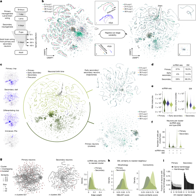
MainThe brain’s ability to process information and produce adaptive behaviours relies on its cellular composition and circuit organization. Throughout development, neurons adopt specific molecular identities that define their physiological function and guide their integration into precise circuit architectures. While spatial and temporal patterning mechanisms coordinating neuronal fate are starting to be elucidated3,4,5, we cannot yet account for the vast cellular complexity of the brain. To gain a comprehensive understanding of how neurons are specified across the nervous system we need systematic, high-resolution characterization of this diversity. Over the past decade, this need has driven two types of large-scale atlasing efforts: single-cell transcriptomics to define molecular identities6,7,8,9,10, and connectomics to reveal anatomical and synaptic relationships of neurons1,11,12,13,14.The dimensionality of these large datasets can be reduced by grouping individual neurons into cell types, which represent the functional units of neuronal circuits14,15,16. In vertebrates, recent mouse and human brain atlases have identified more than 5,000 and 3,000 transcriptional types, respectively6,9. Eventually it will be essential to integrate such molecular taxonomies with other key modalities including neuroanatomy and connectivity15,16. There is currently no clear path to establish a comprehensive correspondence between transcriptomic and anatomical types in vertebrates. However, the situation is more promising for the highly stereotyped and numerically smaller brain of D. melanogaster. In this case, the systematic analysis and annotation of the combined datasets of the central nervous system, the largest connectomes yet completed, revealed over 11,000 neuronal types across 160,000 neurons2,14,17. This complete description of the texture of a complex nervous system provides an exciting opportunity to better understand both the developmental and organizational logic of neural circuits. Nevertheless, comprehensive cross-identification of anatomical and molecular cell types remains challenging.The most complete matching to date has been obtained in sensory systems: for olfactory projection neurons18 and in the visual system (optic lobes)19,20,21,22, where around 800 repeated ommatidia result in hundreds of copies for a relatively small number of cell types. Outside the optic lobes, where most cell types are represented by around 2 neurons per hemisphere, transcriptional coverage becomes a limiting factor: empirical observations and simulation suggest that a minimum of 20–30 cells is needed to identify a cell type in single-cell RNA-sequencing (scRNA-seq) datasets15,23. As a consequence, low-coverage atlases are inherently unsuited to resolve the full connectomic diversity, explaining why large-scale atlases outside the optic lobes24,25,26 reported ten times fewer neuronal types2,14,15. However, high coverage alone might not be sufficient to resolve connectomic types, as work in the olfactory and visual system has shown that transcriptional diversity peaks during development and decreases in adults5,18,20,27, making developmental atlases better suited to capture the diversity in the connectome.Stimulated by these considerations, we have generated a developmental transcriptional atlas of the D. melanogaster ventral nerve cord (VNC), which houses the sensory–motor circuits that form the core interface between the nervous system and the body. The atlas is available for browsing at Scope (https://scope.aertslab.org/#/HundredDrills/*/welcome) and at a dedicated website (https://flyem.mrc-lmb.cam.ac.uk/VNCatlas). Its deep coverage (38× aggregate coverage) enabled high-resolution mapping of neuronal diversity as well as emergent organizational features of molecular identity; comprehensive annotation allowed most cells to be linked to the connectome. Together, these properties of the atlas enabled the identification of a global molecular temporal coordinate system: a sequence of 17 transcription factors (TFs) that define a persistent lineage-independent correlate of neuronal birth order. Comparison of male and female data identified apoptosis and transcriptional divergence as key developmental mechanisms of sex differences and also enabled precise matching with connectomic cell types. This atlas provides a resource and intellectual framework for identifying principles of circuit assembly.Developmental atlas of the nerve cordTo reveal the transcriptional diversity of the 16,000 intrinsic neurons of the VNC, we built an atlas using scRNA-seq (Extended Data Fig. 1). After quality control, we obtained 459,091 cells from four developmental stages (6, 24, 36 and 48 h after puparium formation (h.a.p.f.)), spanning the period when neuronal morphology and connectivity are established28 (Fig. 1a). The atlas includes a balanced number of male and female cells, making it suitable for studying the development and function of sexually dimorphic circuits (Extended Data Fig. 1f).Fig. 1: A developmental atlas of the Drosophila VNC identifies two modes of neuronal diversification.a, Two neurogenic waves in Drosophila development. b, UMAPs showing neurons coloured by stage before (left) and after (right) regression of maturation-driven variability. Insets: the same subsets of cells (i and ii) in either embedding. nSyb expression increases with stage. The dotted line indicates the immature neuron stem region. c, UMAPs for markers of neurogenic wave and maturation status (left). Middle, neurogenic wave and maturation status annotation. Right, UMAPs of primary and secondary neuronal subsets. d, Fractions of primary, secondary and early secondary neurons in the atlas and the connectome. EM, electron microscopy. e, RNA abundance in the atlas (unique molecular identifiers, left) and soma volume in the connectome (right) by neurogenesis wave. f, Neurons per scRNA-seq cluster after normalizing for coverage (24 + 36 + 48 h.a.p.f., 28×) and per connectomic type. g, Constellation plots showing intercluster overlaps. Nodes represent the cluster centroids, and the size is proportional to the cluster size. Brown indicates isolated clusters after weight filtering < 0.1. Edge widths are proportional to the summed bidirectional fraction shared between the two clusters. Given clusters A and B, the edge weight is the fraction of A’s nearest neighbours belonging to B, plus the fraction of B’s nearest neighbours belonging to A. Density plot of the strongest edge for each cluster. n = 627 (primary), n = 365 (secondary) clusters. Statistical analysis was performed using two-sided Wilcoxon rank-sum test; P < 1.3 × 10−14. h, Distribution of NBLAST morphology scores to the top-match neuron (left). n = 1,386, median = 0.45 (primary); n = 9,919, median = 0.55 (secondary). Right, distribution of cosine similarity connectivity scores to the nearest neighbour. n = 1,356, median = 0.55 (primary); n = 9,726, median = 0.74 (secondary). For both comparisons, secondary neurons are more similar than primary neurons. Statistical analysis was performed using two-sided Wilcoxon rank-sum test; P < 2.2 × 10−16. i, Fraction of neurons sharing hemilineage with the kth neighbour at increasing neighbour rank. Black, the same hemilineage; grey, hemilineage identity of neighbour to be determined (TBD).While the atlas contains neurons and glia (see Supplementary Fig. 1 for glia), we focused our attention on the neuronal subset. One of the main drivers of transcriptional diversity is maturation, which results in the layered organization of neurons in uniform manifold approximation and projection (UMAP) space according to the developmental stage at which they were sampled (Fig. 1b). This pattern is mirrored by graded expression of nSyb, a synaptic protein associated with neuronal maturation (Fig. 1b (i and ii)).This embedding captures the molecular dynamics of maturation but it hinders matching cell types across development (Extended Data Fig. 6c). By regressing out maturation-related variability, we integrated transcriptomes from the same cell types across different stages. One exception is the stem region, which contains neuronal precursors and less differentiated neurons from samples from the 6 h.a.p.f. and 24 h.a.p.f. that do not integrate with those from the 36 h.a.p.f. and 48 h.a.p.f. (Extended Data Fig. 2), as those stages lack the corresponding immature cells (Fig. 1b). Our neuronal atlas contains 302,765 cells representing the 7,880 neurons per lateral half of the male VNC connectome (MANC)2, yielding 38× aggregate coverage (per-stage coverage is shown in Extended Data Fig. 1a,f).Two modes of neuronal diversificationIn insects, there are two waves of neurogenesis. Primary neurons are born from stem cell progenitors (neuroblasts) in the embryo where they build the larval brain and are later remodelled through pruning and regrowth of arbours during metamorphosis. The same neuroblasts produce secondary neurons during larval stages, which integrate into adult circuits only in the pupal stage29 (Fig. 1a). We identified primary and secondary populations in the atlas by the mutually exclusive expression of Imp and dati (Fig. 1c) and found primaries segregate into a region of punctate small groupings (clusters) and secondaries into a region of elongated low-dimensional manifolds (trajectories), typically radiating from the stem region (Extended Data Fig. 2). Outside small clusters, we found Imp expression at the tips of trajectories, distal to the stem. These are likely to be the first born neurons produced when the neuroblasts resume division after larval hatching and were annotated as ‘early secondaries’. Neurogenesis wave annotation is supported by the observation that secondary neurons make up 59% of the transcriptional atlas, similar to the 60% reported in a recent scRNA-seq larval atlas30 and to the 66% observed in MANC (Fig. 1d). Moreover, there is a similar trend in cell size, where primary > early secondary > secondary, as measured by number of RNA molecules per cell (transcriptome) and soma volume (connectome) (Fig. 1e).Spatial segregation in UMAP space of primary and secondary neurons highlights neurogenesis wave as a strong driver of transcriptional divergence. However, local organization is also different (puncta versus trajectories) suggesting that these two populations differ in the degree of separation between one cell type and its closest neighbour, with primary neurons diverging more rapidly than secondary neurons. This distinct organization is not an artifact of the joint analysis of primary and secondary neurons, as it is preserved when the two subpopulations are analysed independently (Fig. 1c). Notably, after adjusting for coverage, many primary clusters have sizes compatible with one cell, which is the median number of cells per type in the connectome (Fig. 1f,g), while the median cluster size is three cells. By contrast, secondary neurons yielded a median of 13 cells per cluster at the same clustering resolution, compared to 2 in the connectome (Fig. 1f,g). To better compare primary and secondary neuron clusters, we quantified their degree of similarity using an overlap metric defined as the fraction of neurons of which the nearest neighbours belong to a different cluster. Using this measure, secondary neuron clusters showed greater intermixing than primary clusters, with intercluster relationships forming ordered, trajectory-like structures, in contrast to the more heterogeneous organization of primary clusters (Fig. 1g). This observation aligns with the MANC connectome, in which we find that primary neurons are statistically more distinct from their most similar neighbour than secondary ones (Fig. 1h) and that the nearest neighbour of a secondary neuron is more likely to have the same developmental origin (that is, hemilineage identity) than for primary neurons (Fig. 1i). Together, these results strongly support the idea that secondary neurons diverge more gradually than primary neurons.Hemilineages link the atlas to the connectomeSecondary neurons are born from a defined set of larval neuroblasts (on average 25 per thoracic segment) each defining a stereotyped neuronal lineage. Sibling neurons from each lineage form two hemilineages based on Notch signalling during asymmetric cell division: A (Notch on) and B (Notch off)28,31,32 (Fig. 2a). Crucially, neurons of the same hemilineage bundle together to enter the neuropile, leaving a structural footprint that has been exploited to group them in the connectome achieving over 90% hemilineage annotation coverage2.Fig. 2: Hemilineage and segment annotations link the transcriptome to the connectome.a, Adult VNC showing thoracic (T1, T2, T3) and abdominal (A) segments. 25 stem cells (neuroblasts, NB) per segment generate secondary lineages, their progeny splitting into A and B hemilineages determined by Notch signalling. Male connectome (MANC) renderings for hemilineages 11A and 11B. b, The central UMAP shows hemilineage identity assignments based on cumulative evidence (Extended Data Fig. 4): neurotransmitter predictions, adult VNC scRNA-seq atlas26 annotation, markers from the literature and GFP+ cells from reporter lines in the atlas. Cross-matching between transcriptomic and connectomics atlases is shown for hemilineage 06B (MANC neurons in purple). The fraction of annotated neurons is shown. MNs, motor neurons. c, Precursor cell UMAP with manual annotation based on markers. d, Hemilineage annotation correlation (secondary neurons) between MANC and 48 h.a.p.f. atlas neurons. The dotted grey line indicates identity. e, Expression of Hox genes across segments: canonical (top left) and observed by larval stainings in hemilineages 03B and 07B (top right). Bottom, expression in 03B and 07B secondary neurons at 48 h.a.p.f. The labels show predicted segmental identities. f, Soma segment annotation. GNG neurons are only at 6 h.a.p.f. Inset: MANC 07B secondary/early secondary neurons (left side). The fraction of annotated neurons is shown. g, Segment annotation correlation showing the fraction of secondary neurons per segment per hemilineage annotated in MANC and 48 h.a.p.f. secondary neurons. The dotted grey line indicates identity. The solid red line is the fitted linear model. h, UMAP of secondary neurons colour-coded by hemilineage trajectory complexity (top). Bottom, the per-hemilineage proportion of secondary neurons with serial homologues in MANC coloured by trajectory complexity. Trajectory complexity in the atlas is significantly correlated with intersegmental homology in the connectome. Statistical analysis was performed using the one-sided Jonckheere–Terpstra test; P = 2 × 10−4. A neuronal type with serial homologues across thoracic segments is shown as an example. i, Antp expression at 6 h.a.p.f. per hemilineage across segments and coloured by trajectory complexity. Hemilineage order is as in h.As hemilineage identity is one of the main sources of transcriptional heterogeneity in the VNC26, we examined whether the trajectories in UMAP space reflected hemilineage identity. First, we assigned neurotransmitter identity, as neurons from the same hemilineage share neurotransmitter use2,33,34. We found that cells in each trajectory expressed primarily just one fast-acting neurotransmitter (Fig. 2b and Supplementary Fig. 2), supporting the idea that trajectories represent hemilineages.To provide direct experimental evidence for hemilineage identity, we included samples from four GFP reporter lines that label specific hemilineages (09A, 01+10B, 07B, 08B+09B)35 throughout development and into adulthood; the distribution of GFP-positive cells along specific trajectories confirms that trajectories correspond to hemilineages (Fig. 2b). We next used multiple sources of evidence (Fig 2b and Extended Data Fig. 3a) to annotate hemilineage identity for over 95% of secondary and 44% of primary neurons, linking them to groups of, on average, 153 neurons and 60 neuronal types in the connectome (for example, 151 neurons and 49 types in 06B). We next extracted markers for hemilineage identity, of which 88% were TFs (Extended Data Fig. 3b), and Notch status (Supplementary Fig. 3). We found that 15 out of 34 hemilineages can be distinguished by the expression of a single marker, while the rest are identified by marker combinations; these markers provide genetic access to hemilineages and helped extend hemilineage annotation to neurons in the stem region, poorly predicted by our annotation pipeline (Fig. 2c).The accuracy of our atlas annotation is supported by a very strong correlation between the observed sizes of hemilineages in the atlas and the connectome (R2 = 0.9; Fig. 2d).Segmental identity links the atlas to the connectomeLike the vertebrate spinal cord, the VNC has a repeated segmental organization: homologous lineages are generated across segments, acquiring segment-specific characteristics through anteroposterior patterning specified by gradients of Hox gene expression36,37 (Fig. 2a). To assess the impact of segmental organization on the transcriptome while refining our transcriptome–connectome matching, we combined Hox gene expression in the atlas with Hox protein expression in larvae to annotate segments across hemilineages (Fig. 2e and Extended Data Fig. 4a–c). In total, we provide segment identity predictions for 94% of secondary neurons and 43% of primary neurons (Fig. 2f; annotation validation is shown in Supplementary Fig. 4).The intersection of hemilineage and segment predictions subsets the atlas into 122 groups of secondary neurons, each mapping onto a mean of 51 neurons or 26 types in the connectome. The quality of the matching is supported by a strong correlation between the fraction assigned to each group in either dataset (R2 = 0.71; Fig. 2g).For some hemilineages, intersegmental differences are large, resulting in independent trajectories each displaying specific marker genes (such as 03B), while others overlap partially (01A) or completely (13A) (Fig. 2h, Extended Data Fig. 5 and Supplementary Fig. 4). This difference in trajectory complexity could underlie the different degree of neuronal intersegmental (serial) homology observed in the connectome (for example, IN13B005 type has serially homologous neurons in all three thoracic segments; Fig. 2h). To test this, we classified hemilineages into three categories of complexity: low (fully overlapping), medium (partially overlapping) and high (non-overlapping). We found that the transcriptional categories are significantly linked to the degree of intersegmental homology reported in the connectome2,38 (Fig. 2h). Notably, Antp is expressed across the three segments in low-complexity hemilineages, instead of the expected restriction to T2 (Fig. 2i and Extended Data Fig. 4b), suggesting that Antp may contribute to reinforcing neuronal homology across thoracic segments. This might be needed to obtain neuronal identities implementing segmentally repeated sensory–motor circuits (for example, leg movement).A global temporal code for birth orderSequential generation of different neuronal types from shared progenitors is a core developmental feature of the insect central nervous system39,40 and other systems, such as the mammalian retina41. Notably, the expression patterns of Imp (confined to the tip of trajectories opposite to the stem; Fig. 1c) and of known genetic markers of birth-order identity42,43 (mamo, jim and br) (Fig. 3a and Extended Data Fig. 6a) provide strong evidence that neurons are arranged along trajectories according to their birth order. Neuronal diversity within lineages should therefore result from changes in gene expression along each trajectory (Fig. 3a). Using trajectory inference analysis, we identified a total of 1,508 genes differentially expressed along trajectory pseudotimes for all hemilineages, of which 149 were TFs (Fig. 3b,c). Notably, 40 of those TFs were common to more than 50% of the hemilineages, raising the possibility of a shared temporal program across hemilineages. This was supported by the observation that some TFs were expressed in a conserved order across lineages and invariant through developmental stages when assessed relative to bona fide cell-type-specific markers such as neuropeptides (Fig. 3d and Extended Data Fig. 6b,c).Fig. 3: 17 TFs define a global temporal code of neuronal birth order.a, Within hemilineages, cell types are born sequentially (left). Right, hemilineage 10B-T1 UMAPs showing three consecutive birth-order markers. b, Fitted trajectory and pseudotimes for 03A-T1 and 6 DEGs. c, DEGs with q < 0.01 and Moran’s value > 0.3 along trajectories. The distribution of DEGs across gene categories (pie chart) and hemilineages (histograms) are shown. Each bar represents genes shared by that number of hemilineages. Grey, DEGs; blue, TFs; red, cell surface molecules (CSM); brown, dual function. d, Normalized expression profile along pseudotime for 6 TFs that are differentially expressed in 95% of hemilineages. Dashed lines link expression peaks. The asterisk indicates the peak that is absent in 06A-T1. e, Expression profiles of CG7368 along pseudotime for 06A-T1 before and after alignment (left) and across trajectories after alignment (right). The average expression profile and average peaks are shown in brown. f, CG7368 normalized expression along pseudotime in trajectories before (left) and after (right) alignment. The y axis dot colours represent hemilineages from Fig. 2 (left) and segments (right; green, T1; blue, T2; and purple, T3). g, TFs expressed in a shared temporal order across lineages (shTFs). Top, for 03A-T1, the normalized expression along pseudotime of shTFs ordered by the first peak in the consensus sequence. Bottom, aligned gene expression peaks positions arranged by consensus order. Each dot is a peak in a single trajectory. The coloured peaks match the average active peak (the intensity represents the detection frequency across trajectories) and the grey peaks represent other peaks. h, Specific adult neuronal populations labelled by danr–hemilineage-specific marker intersection. The UMAPs represent cells co-expressing hemilineage markers (ap for 04B and dmrt99B for 13A) and danr. Maximum-intensity projection of confocal stacks registered to the VNCIS2 template: split-GAL4 intersection patterns in adult VNCs. The numbers indicate the average hemilineage neurons labelled per side ± s.d./average MANC hemilineage neurons per side. The arrowheads indicate neurons belonging to the expected hemilineage. In agreement with atlas predictions, clusters not belonging to 04B or 13A are visible, likely primary neurons.To facilitate a direct comparison of gene expression dynamics across hemilineages and segments, we aligned all trajectories to a single reference trajectory—03A-T1, one of the longest continuous trajectories in the atlas (Fig. 3e and Extended Data Fig. 6d,e). This shared space enabled us to identify expression peaks that are aligned in pseudotime across hemilineages and segments (Fig. 3e,f). As a result, we found 17 TFs that exhibit a conserved pattern of expression along pseudotime and across hemilineages (hth, chinmo, pdm3, pros, ab, mamo, CG7368, rn, CG3726, jim, br, dati, Eip93F, bab1, bab2, danr and dan) (Fig. 3g and Supplementary Fig. 5), hereafter referred to as shared TFs (shTFs). Several shTFs are expressed multiple times along trajectories, expanding the number of conserved expression peaks to 33 (Fig. 3g). Most shTFs show persistent expression throughout developmental stages (Extended Data Fig. 6f) and we confirmed protein expression in adults for nine of them (Hth, Bab1, Bab2, Dan, Br, Eip93F, Mamo, Pdm3 and Pros), in both the VNC and central brain (Extended Data Fig. 7). Thus, the combinatorial action of shTFs offers a possible mechanism to generate neuronal diversity. Moreover, the intersection of shTFs expression with hemilineage-specific markers could be turned into a modular genetic approach to access cell types. We confirmed this possibility by labelling small populations of neurons born during the danr temporal window from hemilineages 04B and 13A in adults using the split-GAL4 system (Fig. 3h).To validate that shTF expression is locked to neuronal birth time, we performed pulse–chase labelling, in which larvae were fed EdU during non-overlapping time windows (Fig. 4a). We found that neurons expressing shTFs from non-overlapping temporal domains in the atlas (br and bab1; Fig. 4b,c) are born in distinct temporal windows in the larva: Bab1+ cells are born in early and late windows, while Br+ cells are born in between (Fig. 4d), consistent with their expression in the atlas.Fig. 4: The VNC’s global temporal transcription code is conserved in the brain.a, EdU pulse–chase experiments. h.a.l.h., hours after larval hatching. b, EdU-labelled (green) VNCs from larvae fed during the 93 h.a.l.h. window, together with Br (magenta, left) or Bab1 (magenta, right). Whole VNCs are displayed as maximum-intensity projections. Insets: single z plane and the corresponding segmentation results for EdU (top), shTF (middle) and their intersection (bottom). Scale bars, 50 µm. c, Expression along pseudotime for br (blue) and bab1 (red) in hemilineage 03A-T1. d, Fraction of shTF+ cells colocalizing with EdU across feeding windows (see the ‘EdU labelling’ section of the Methods). Each dot represents one VNC (n = 2–4 per condition). e, Overexpression (OE) of Br-Z4 isoform in hemilineage 14A causes the disappearance of Bab1+ cells within 14A and a change in projections morphology. Projections lost (yellow) or gained (cyan) in the Br-Z4-overexpression condition are marked by arrowheads. Whole VNCs are displayed as maximum-intensity projections. Insets: a single z plane. Scale bars, 20 µm. Images are representative of n = 4 per condition. f, Connectomic (MANC) types lost (left, yellow arrowheads) or gained (right, cyan arrowheads) by Br-Z4 overexpression. g, Rendering of the brain highlighting regions of origin for the hemilineages examined in h. h, Expression of shTFs for hemilineages in the brain as in Fig. 3g. GNG data from 6 h.a.p.f. and SLP data from 6–48 h.a.p.f. LB, labial; MX, maxillary; MD, mandibular. i, shTFs expression correlation between the reference trajectory (03A-T1) and aligned trajectories from brain (h) or VNC. Each dot represents the mean correlation across 17 shTFs for a hemilineage–segment combination (n = 4 CB, 89 VNC). The plot shows the median of the mean correlation ± interquartile range (IQR); the whiskers extend to the most extreme datapoints within 1.5 × IQR. Shuffled, correlations were calculated by shuffling shTF identity 200× per hemilineage. Statistical analysis was performed using two-sided Wilcoxon rank-sum tests; *P = 0.029, ****P < 2 × 10−16; NS, P > 0.5.Broad defines neuronal identityThe persistent expression of shTFs suggests they may act as terminal selector genes44. We tested this possibility by looking for changes in neuronal identity when ectopically expressing Br outside of its temporal window in hemilineage 14A. We used Bab1 expression as a readout of genetic interaction between shTFs expressed in non-overlapping temporal windows (Fig. 4c) and found that, while it is readily detected in control animals, ectopic Br expression eliminates Bab1 expression within 14A neurons (Fig. 4e). Furthermore, some neuronal processes are substantially reduced, while others are enhanced (Fig. 4e), with no significant changes in the number of neurons (mean ± s.e.m. in thoracic segment 1 (T1), overexpression, 152 ± 1.5, n = 4; control, 155.3 ± 2.0, n = 3; two-tailed Student’s t-test, P = 0.23). Notably, in the MANC connectome, we identified 14A neuronal types compatible with the lost or gained processes (Fig. 4f). We conclude that ectopic Br expression is sufficient to shift neuronal identity within the 14A hemilineage, supporting a role as a terminal selector in the VNC.The shTF code is conserved in the brainWe examined whether the shTF code extends to secondary neurons in the brain by analysing a small subset of hemilineages in two brain regions: the gnathal ganglia (GNG), evolutionarily linked to the VNC, and the superior lateral protocerebrum (SLP), a more derived region without clear transcriptional, morphological or functional homology to the VNC45 (Fig. 4g). For the GNG, we used trajectories present in 6 h.a.p.f. samples due to imprecise separation of brain and VNC tissues (Extended Data Fig. 4d,e), while the SLP hemilineage was isolated from an independent brain dataset (Methods).In both regions and across all four hemilineages, shTFs exhibited expression patterns consistent with those observed in the VNC (Fig. 4h). We quantified this observation by calculating expression correlation between each hemilineage and the 03A-T1 reference. We did not observe a statistically significant difference between brain and VNC scores (Fig. 4i), supporting the notion that shTFs influence the development of all secondary neurons in the central nervous system, excluding the optic lobes.Sex differences across the nerve cordMany aspects of sexually dimorphic behaviours are implemented by neural circuits in the VNC, such as courtship song production in male flies or post-mating behaviour in female flies46. VNC connectomes for both sexes enable comparative analysis and the identification of dimorphisms at scale17, of which the origin and nature could be elucidated by adding developmental molecular information.The balanced number of cells per sex in the atlas enabled us to identify regions displaying differential abundance, containing 4.3% of the neurons at 48 h.a.p.f. (Fig. 5a,b and Extended Data Fig. 8a). Male-enriched cells are more likely to be secondary neurons (81%), while female-enriched cells are biassed towards primary neurons (78%) (Fig. 5b) and these differences correlated with the expression of the key sex-determination genes fruitless (fru) and/or doublesex (dsx)46 (Fig. 5b).Fig. 5: The transcriptional atlas predicts sex differences between male and female connectomes.a, UMAP of differentially abundant regions per sex at 48 h.a.p.f. (blue, male enriched; orange, female enriched). b, Percentage of neurons enriched per sex at 48 h.a.p.f.; percentage of primary and secondary neurons in sex-enriched regions; and fru and dsx expression in sex-specific neighbourhoods at 48 h. c, Beeswarm plots showing the secondary neuron differential abundance at 48 h.a.p.f., grouped by hemilineage and soma segment. Each dot corresponds to a neighbourhood in miloR analysis, coloured by mean fru expression. The boxes show hemilineages proofread in FANC. FC, fold change. d, Pipeline for matching the MANC and FANC connectomes. e, Proofread hemilineage annotation in FANC. Bottom, neurons per hemilineage, per side, per sex after proofreading (L, left; R, right). Top, the number of MANC neurons belonging to types for which FANC matches were not found by the automatic pipeline. Inset: 08B-T2 manually curated neurons in MANC (green, left) and FANC (magenta, right) in MANC space. f, Pipeline to identify candidate fru+ neurons in MANC starting from MARCM clones. g, The atlas predicts sex-specific and shared fru+ neurons in the connectome. Top, 48 h.a.p.f. secondary 08B-T2 neurons arranged by pseudotime and coloured by vPr-l clone. Bottom, vPr-l neurons in the connectome. Green, MANC; magenta, FANC. Left, male-specific neurons. Right, shared neurons. n values indicate the number of neurons. h, fru (left) and rpr (right) expression in 08B-T2 secondary neurons along pseudotime, split by sex and stage. i, Male and female dimorphic fru+ neurons. j, UMAP showing 01A-T1 secondary neurons at 48 h.a.p.f. Colours represent fru expression, cluster identity calculated using shTFs, the number of DEGs per cluster, sex and per-cell correction score after sex regression. k, Molecular differences at 24 and 48 h.a.p.f. Average correction score per cluster (top). Number of DEGs between male and female per cluster (bottom). The lines connect corresponding clusters. Green or blue lines indicate P < 0.01, as calculated using two-sided Student’s t-test with Bonferroni correction. n > 26.Among the well-annotated secondary neurons, sexual dimorphisms map to a small number of hemilineage–segment combinations (Fig. 5c and Extended Data Fig. 8b,c). We validated our predictions in the male (MANC) and female (FANC) connectomes, focussing on six hemilineage–segment combinations: 08B-T1 and 08B-T2 (male enriched), 01A-T1 (reported sexually dimorphic47) and 01A-T2, 06A-T1 and 06B-T1 (isomorphic) (Fig. 5c). We established an automated pipeline to obtain one-to-one matching between MANC and FANC neurons and transfer hemilineage labels from the well-annotated MANC to FANC (Fig. 5d and Methods). As predicted by the atlas, we found the greatest numerical differences in 08B-T1 and 08B-T2, which also had the largest number of MANC-specific neuronal types (Fig. 5e).While not all fru+ neurons belong to numerically dimorphic groups (Extended Data Fig. 8d), nearly all sex-biased secondary neurons expressed fru (Fig. 5c). We mapped these neurons in the MANC connectome using published light-level images of fru+ lineage-related neurons (MARCM clones)47 (Fig. 5f and Supplementary Table 2). By linking gene expression, hemilineage identity and neuronal morphology, we matched small groups of fru+ neurons across the atlas and the connectome (Extended Data Fig. 9). To validate our annotations we focused on fru+ neurons from hemilineage 08B-T2, which we mapped to the vPr-l clone. In the atlas, vPr-l neurons are born at three pseudotime windows: most are early born and male specific, while two later-born small groups have neurons from both sexes (Fig. 5g). Consistent with this, in the connectome, most vPr-l types are male specific, with only two types (three neurons per side) shared between sexes (Fig. 5g). Furthermore, MANC–FANC matching and intersectional labelling experiments confirmed atlas predictions of male-specific hemilineage 04B neurons in all thoracic segments, despite a corresponding clone (vPr-g) reported only in T147 (Extended Data Fig. 8e,f). Notably, 04B fru+ neurons are late born in the atlas, consistent with the external position of male-specific vPr-g cell bodies in MANC (Extended Data Fig. 8e). These results showcase the atlas’s power for studying known and previously unknown sexual dimorphisms.Molecular mechanisms shaping dimorphismWe next examined how sex differences emerge during development. The atlas shows that dimorphisms develop progressively throughout metamorphosis (compare Extended Data Fig. 10a and Fig. 5c). Accordingly, neurons within the vPr-l male-specific temporal window are gradually lost in females through pupal development. This correlates with increased expression of the pro-apoptotic gene rpr at 24 h.a.p.f. only in females (Fig. 5h and Extended Data Fig. 10b), suggesting that female-specific apoptosis causes the imbalanced cell number. Regions of female-specific apoptosis are present across the atlas (Extended Data Fig. 10c), pointing to its widespread role in shaping male-specific domains, extending earlier results in the brain48,49.While some neurons are sex specific, others only show morphological differences47. To investigate the molecular signatures underlying morphological dimorphisms we focused on hemilineage 01A-T1, in which we mapped previously described sex differences in the dPr-a fru+ clone47 to both MANC and FANC connectomes (Fig. 5i). The atlas shows that fru+ neurons display a clear separation between males and females in 01A-T1 UMAP space (Fig. 5j). We calculated gene expression differences between sexes in clusters of the 01A-T1 lineage and identified the dimorphic cluster to have the highest number (Fig. 5j). Notably, among the most significant genes, we found several with synaptic partner matching functions, such as members of the beat, side and dpr families50 (Extended Data Fig. 10d), that might have an instructive role in dimorphic wiring. Finally, we quantified the emergence of dimorphism through metamorphosis, by defining a per-cell male–female molecular distance metric (Fig. 5j and Methods). This shows that molecular distance, and the number of differentially expressed genes (DEGs), increase with developmental time specifically in fru+ neurons (Fig. 5k).Overall, these results show that sexual dimorphisms emerge through development from neurons with the same temporal origin by using two alternative strategies: sex specific apoptosis and transcriptional divergence. Two recent independent studies reached similar conclusions that sexual dimorphisms reflect sex-specific developmental programs acting on neurons born in the same lineage and birth order, rather than de novo generation of sex-specific cell types51,52.DiscussionHere we report a high-resolution developmental transcriptional atlas of the Drosophila nerve cord. This provides a platform to investigate the molecular logic of the thousands of cell types that wire up to form the sensory–motor circuits in the nerve cord, similarly to how more focussed atlases within the brain have been used to understand wiring specificity of Drosophila olfactory53 and visual circuits54,55,56. To facilitate exploration, our data are available at Scope (https://scope.aertslab.org/#/HundredDrills/*/welcome) for gene expression browsing, and on a dedicated website (https://flyem.mrc-lmb.cam.ac.uk/VNCatlas), which integrates transcriptomic and connectome metadata. We linked the atlas and the connectome by sequentially annotating primary and secondary neurons, hemilineages, segments and fru expression. Our description of molecular identity of consecutively born secondary neurons opens the possibility for alignment of transcriptomic and connectomic types. Comparative analysis of sexual dimorphisms in fru+ neurons refined cross-matching with the connectome to as few as three neurons (Fig. 5g). While exhaustive cross-annotation is a future goal, this correspondence for fru+ neurons shows that our atlas contains sufficient information for identification of precise connectomic cell types. Stochastic labelling of neuronal morphology39,40, or dense labelling of shTFs coupled with light-microscopy-based connectomics (LICONN)57 are promising avenues for full-scale alignment with the connectome.Our data show that the molecular profile of consecutively born neuronal types diverge much more gradually in the larva than the embryo. Increasing the coverage of the atlas will establish whether secondary types indeed resolve in fully isolated clusters. Notably, the temporal patterning mechanisms specifying embryonic-born versus larval-born neurons mirror this distinct organization: a discrete temporal cascade of TFs in embryonic neuroblasts4,58,59 versus opposing gradients of the RNA binding proteins Imp (early) and Syp (late) in larval neuroblasts60,61. The relationship between temporal origin and molecular identity has been characterized in embryonic and optic lobe neurons4,62, but how Imp/Syp gradients translate to neuronal identities is only starting to be explored42,60,63. We propose that, by encoding a persistent molecular timestamp of neuronal birth order, the 17 shTFs are perfectly poised to be key intermediaries in this process. Although the precise functional contributions of most shTFs in specifying and maintaining neuronal identity remain unresolved, instructive roles in fate specification have been identified for some21,52,64,65. Our Br overexpression confirms this role in the VNC. From an evolutionary perspective, a gradual molecular identity system could offer several advantages. It is more evolvable, as small shifts in gene regulation can generate new neuron types without requiring new patterning modules, enabling gradual diversification and behavioural adaptation.The shTFs that we identify are reminiscent of concentric genes demarcating successive cohorts of neurons in the Drosophila optic lobe22,62,66. However, the shTF code operates in the central brain and VNC, in which there are over 10,000 cell types in contrast to a few hundred intrinsic cell types in the optic lobe13. Our atlas provides the strongest evidence to date for a persistent molecular correlate of birth order operating across secondary neurons, extending temporal logic beyond previously studied, region-specific systems22,27,42,62,66. Consistent with our findings, nine shTFs had previously been identified as markers of specific projection neuron (PN) types27. In this context, br and Eip93F label mid-born projection neurons, whereas danr marks late-born projection neurons. Moreover, two recent studies have identified most shTFs in a small subset of central brain hemilineages in pupae and adults52,67 (Supplementary Table 3). However, beyond the 17 shTFs, other TFs identified in those studies are not broadly shared across lineages and therefore do not meet our inclusion criteria for shTFs.Notably, the temporal specification of neurons in flies has parallels in mammals. Homologues of Imp and Syp exist and have been implicated in neurogenesis68,69. Furthermore, a shared transcriptional code has recently been described in maturing neurons of the mouse spinal cord, where early neurons express Onecut family TFs, intermediate neurons express Pou2f2, Zfhx3 and Zfhx4, and late-born neurons express Nfia and Nfib, often in combination with Neurod2 and Neurod670,71. This evidence points to an evolutionarily conserved temporal logic governing the generation and organization of neuronal diversity.This shared code is likely to result from the common evolutionary origin of progenitors and its conservation suggests functional importance. Shared temporal modularity could ensure stepwise circuit assembly and wiring coordination in local neuronal domains, as shown for local premotor circuits72, or between distant brain and VNC regions. This opens paths to study the idea that “neurons that are born together wire together”73. The recurrent expression of the same TF in neurons from different temporal windows could be responsible for reoccurring morphological features in temporally distant neurons within lineages39,40. Notably, six shTFs have roles specifying distal structures (hth74, dan, danr75, bab1, bab2, rn76). Proximal–distal patterning has a temporal component, with positional identity being the result of the timing of exposure to spatial patterning factors. This suggests that regulatory networks may be repurposed in different developmental contexts or a deep common evolutionary origin for neuronal and non-neuronal tissue patterning.Many additional insights remain latent in the atlas, which will be a valuable resource not only for the Drosophila neuroscience community, but also for comparative studies exploring the evolutionary origins of neuronal diversity and function across phyla. It also provides a strong motivation to obtain a correspondingly high-coverage developmental brain atlas to complete the molecular description of the fly central nervous system.MethodsscRNA-seq data generationTo discriminate technical from biological variability, we used flies from different genetic backgrounds19,77, enabling us to generate scRNA-seq libraries of VNCs of different sex and developmental stages and separate them after sequencing through single-nucleotide polymorphisms (SNP)-based sample demultiplexing (see below)78 (Extended Data Fig. 1). Randomized samples from different genotypes were used for the same sex and developmental stages across experiments. In total, data were collected from 92 individual animals, covering four developmental stages and both sexes. Each stage–sex condition is represented by 5 to 18 biological replicates, covering between 5 and 11 different genotypes. Some experimental preparations were used to create 2 or 3 independent libraries.DissociationFor each stage–sex condition, several genotypes and individuals were used, as summarized in Supplementary Table 1. Flies of the genotypes indicated in Supplementary Table 2 were allowed to mate and their larvae developed at 25 °C until white pupae stage. Then pupae were collected with forceps, sexed under a dissecting scope and put in either male or female vials to develop until the correct stage, that is, 6, 24, 36 or 48 h.a.p.f. VNCs were dissected in ice-cold DPBS (Dulbecco’s PBS, Gibco). A maximum of 8 VNCs, each of a different genotype, was pooled in a low-bind Eppendorf tube containing 100 µl of DPBS on ice. VNCs from animals of two or three different developmental stages and sex were pulled in the same tube (6 + 24 h.a.p.f., 24 + 48 h.a.p.f. or 24 + 36 + 48 h.a.p.f.). Four brain samples were included in the last round of experiments, but later excluded from the analysis of VNC. After dissections, tissues were collected at the bottom of the tube by centrifugation (800g, 5 min, 4 °C), DPBS was replaced with 50 µl of dispase I (3 mg ml−1, Sigma-Aldrich, D4818, reconstituted in 50 mM HEPES/KOH pH 7.4, 150 mM NaCl) and 75 µl of collagenase I (100 mg ml−1, Invitrogen, 17100-017, reconstituted in HBSS). VNCs were dissociated in a thermo mixer (Eppendorf) at 25 °C at 500 rpm for 30 (6 + 24 h.a.p.f. samples) or 40 min (24 + 36 + 48 h.a.p.f. samples). Dissociation was aided by pipetting up and down 10 times every 10 min ensuring that the tip touched the bottom of the tube to increase the mechanical stress. Dissociated cells were centrifuged (800g, 5 min, 4 °C), washed once with DPBS and resuspended in 180 µl of DPBS with 0.04% BSA. The cell suspension was filtered through a 10 µm filter (pluriStrainer, Cambridge Bioscience, 43-50010-03). Viability, presence of debris and cell number were accessed using the Countess II automated cell counter (Invitrogen).Library preparation and sequencingSamples were collected on 3 different days. Each day, a total of 4 different cell suspensions (independent samples) was generated, each containing different combinations of genotypes, ages and sex. Single-cell expression libraries were generated at the CRUK-CI sequencing facility using Chromium Next GEM Single Cell 3′ HT v3.1. We aimed to load each sample in duplicate, 20,000 cells per lane. Before sequencing, libraries were inspected on the TapeStation. Sequencing was performed on the NovaSeq6000 machine (Illumina) with the following sequencing parameters: 28 regular cycles of which 16 are 10x barcode and 12 are unique molecular index, 10 i7-index cycles, 10 i5-index cycles, 90 regular cycles.scRNA-seq data processingNo formal experimental blinding was applied for the generation and analysis of the scRNA-seq atlas; however, computational analyses were performed in an unsupervised manner, and clustering and dimensionality reduction were performed without using sample identity.CellRangerData from the NovaSeq6000 sequencer were processed using CellRanger v.8.0.0 using the cellranger count function with the default parameters. CellRanger reference index genome was built on genome assembly BDGP6.32 supplemented with the coding sequences for the expected transgenes (Supplementary Table 6). Before quality control, cell ranger total output was 805,970 cells. The median sample number of reads per cell was 39,142, the number of detected genes per cell 1,511 (min = 183, max = 8,543) and the median number of unique molecular identifiers (UMIs) per cell 4,893 (min = 666, max = 847,868).DemultiplexingThe output from CellRanger was demultiplexed using applications from the Demuxafy docker container v.3 (https://demultiplexing-doublet-detecting-docs.readthedocs.io/en/latest/index.html)79. SNP information for all sequencing reads (Pileups) were generated using cellsnp-lite (v.1.2.3) with the parameters ‘--chrom 2 L,2 R -p 22 --minMAF 0.1 --minCOUNT 100’. Out of the 4 fly chromosomes, only chromosome 2 was used for demultiplexing because, in our cross schemes, it always comes from the DGRP lines, while the remaining chromosomes originate on the other stocks. The demultiplexing package Vireo78,79 was run twice on the pileups, once using a variant call format (VCF) reference file and once without it (withVCF and noVCF in Extended Data Fig. 1). The VCF file for the first run was generated using the DGRP SNP data from the Aerts laboratory (https://resources.aertslab.org/DGRP2/NCSU/final/dm6/DGRP2.source_NCSU.dm6.final.SNPs_only.vcf.gz). The parameters used were ‘-N noSamples -p 4 --randSeed=1’ where noSamples is the number of different genotypes present in the given sample. The noVCF run can identify all genotypes in an unbiased way but does not provide the identity of the groups, that is, while it produces groups 1 to 7, it does not indicate which genotype each group corresponds to. Conversely, the run withVCF can identify most genotypes but is less efficient in identifying singlets due to the variable quality of VCF information across DGRP genotypes and the confounding effect introduced by DGRP heterozygosity of chromosome 2 (only one parent carried the DGRP chromosome). To use the demultiplexing results of the more efficient noVCF runs, we used several source of information to assign groups to genotypes: (1) the correspondence between expected sex and roX1 expression; (2) expression of GFP transgenes; and (3) comparison of the results from noVCF and withVCF Vireo results (Extended Data Fig. 1). In the rare cases in which the genotype assignment provided by the withVCF run disagreed with the sex or GFP transgene expression, these took precedence. Besides enabling assignment of metadata information such as sex and stage of the cell, demultiplexing also enabled removal of doublets, given that those cells have a high fraction of SNPs coming from different DGRP lines. Cells were considered doublets if they were classified as such in the Vireo noVCF run and excluded from further analysis.Gene annotationsThe list of TFs comprises the union of genes annotated as TFs in flybase and TFs reported previously80. Annotation of cell surface molecules was taken from ref. 80. Genes involved in cellular energy production and stress response correspond to the union of flybase gene lists: CYTOCHROME_C; ELECTRON_TRANSFER_FLAVOPROTEINS; MITOCHONDRIAL_COMPLEX_III; MITOCHONDRIAL_COMPLEX_II; MITOCHONDRIAL_COMPLEX_IV_CYTOCHROME_C_OXIDASE_SUBUNITS; MITOCHONDRIAL_COMPLEX_I_SUBUNITS; MITOCHONDRIAL_COMPLEX_V_ATP_SYNTHASE_COMPLEX_SUBUNITS; heat_shock_prot.Quality controlThe Cell ranger output was imported into an R object using sequentially the functions Read10X and CreateSeuratObject from the Seurat package (v.4)81 with the default parameters. Some of the last analyses were performed using Seurat (v.5)82. A first quality-control filter was applied to exclude cells with fewer than 700 features, more than 20% of mitochondrial genes and more than 50% of ribosomal genes. Genes expressed by fewer than three cells in the dataset were also excluded. Samples showed a bimodal distribution of UMIs and features across cells, except for SITTD8, for which the distribution was unimodal. For this reason, we excluded SITTD8 from further analysis.Data integrationData integration was performed twice following the same pipeline (see below) to integrate the full dataset (including neurons and glia) as well as the subsets containing either neurons or glia.Data integration was performed using the rpca algorithm in Seurat. In brief, 3,000 features were found using SelectIntegrationFeatures, FindIntegrationAnchors was then run on those features using the 24 h.a.p.f samples as reference and lastly, the anchors were used with the IntegrateData function with a k.weight = 100 (or number of cells −2 for small samples). This integration process removes variability due to stage and genotype. Cells with fewer than 3,000 UMIs or in clusters with an average number of UMIs smaller than 3,000 were excluded from further analysis as these were deemed to be low quality. The resulting VNC dataset has a median of 23,976.3 UMIs (min = 3,000, max = 565,460) and a median number of genes of 3,445 (min = 731, max = 8,428).Atlas annotationNeurons and gliaTo annotate neurons and glia we calculated, using the Seurat function AddModScores, enrichment scores for glial (wrapper, repo, CIC-a, loco, CG10702, CG6126, Gs2, Egfr, Tret1-1, bdl, Zasp52, rols, ine, CG5404, CG14688, CG31663, ry, CG4752, betaTub97EF, CG32473, LManII, Eaat1, alrm, Eaat2, axo, Vmat, moody, Indy, zyd), neuronal (elav, nSyb) or ‘other’ (CG11835, alphaTub85E, Act57B, betaTub60D, CG5080) marker genes. Markers for the category ‘other’ were chosen for being specifically expressed in a cell population lacking neuronal as well as glial markers. Gene Ontology analysis identified several genes enriched in cells of mesenchymal origin among markers for the other category. Categorical assignment of cells to glia, neuron or other was done based on a cluster-based winner-takes-all criterion. The category ‘other’ was excluded from any further analysis.Glia typesGlial clusters were annotated according to the expression of previously reported markers83. Specifically sim expression was used for midline glia, CG6126 for MAP, ltl for subperineurial, alrm and Tre1 for astrocytes, wrapper for cortical and axo for ensheathing glia. Similarly to neurons and glia, glial identity was assigned based on a cluster-based winner-takes-all criterion.Neurogenesis wave and maturation stateThe adult brain contains primary neurons, born in the embryonic phase, and secondary neurons, born during larval stages. To identify these distinct populations in our atlas, we used the markers Imp (primary) and dati (secondary)30,60,84. First we assigned categorical identity to neurons expressing high levels of markers (primary, Imp > 2; secondary, dati > 2 in the stage-integrated data slot), producing nearly completely mutually exclusive labels. We reasoned that neurogenesis wave information might be more prominent in earlier developmental stages and used the obtained labels to train a classifier using the devCellPy machine learning framework85 with parameter rejCutoff = 0.5 and testSplit = 0.1. The trained model was used to predict primary and secondary labels across the atlas. Expression data for training and classification included all 3,000 genes from the stage-integrated data slot.The stem region of our atlas contains cells with low expression of dati and markers of mature neurons, such as brp and nSyb, and it is devoid of 36 h.a.p.f. and 48 h.a.p.f. cells, suggesting it corresponds to neuronal precursors. We annotated these neurons using a similar strategy as above, but using brp (>1.5) for mature neurons and the chromatin remodelling factor Phs (>1.5) for immature ones. Similarly to the neurogenesis wave, we trained the classifier on 6 h.a.p.f. data and then used the model to predict labels across the atlas. In both cases, training and prediction were performed 50 times starting from the same training set and the consensus result was used for the final assignment.Cell cycle phaseCell cycle annotation was done using the Seurat function CellCycleScoring. Marker genes for the different phases of cell cycle were obtained from ref. 86.Neurotransmitter identityEach neuron in the atlas was assigned a fast neurotransmitter identity based on the highest expression level among the markers VAChT (cholinergic), Gad1 (GABAergic) and VGlut (glutamatergic). Neurons were assigned a monoamine class (tyraminergic, octopaminergic, dopaminergic, serotonergic and histaminergic) if they co-expressed the vesicular monoamine transporter (Vmat) and monoamine-specific markers (tyramine: Tdc2+, Tbh−; octopamine: Tdc2, Tbh; dopamine: Ddc, ple; serotonin: Trh, Ddc; histamine: Hdc).HemilineageTo provide experimental evidence for hemilineage assignments, we included among the sequenced samples transgenic lines in which GFP expression is specifically driven in lineages/hemilineages (09A, 01+10B, 07B, 08B+09B). This was obtained either through split-GAL4 intersectional approach (09A, line 1, Dr-AD/Gad1-DBD; 08B + a subset of neurons from 09B, line 4, Lim3-DBD/c15-AD)35,87,88 or through an immortalization-based strategy (01+10B, line 2, R16A05-AD;R28H10-DBD; 07B, line 3, Dbx-DBD/ey-AD)31,89.Annotation of hemilineages was performed using a stepwise approach, integrating information from multiple published and unpublished sources (summarized in Supplementary Table 4). We first assigned hemilineages with strong supporting evidence from previous studies, which helped to reduce the number of unassigned orphan hemilineages requiring further annotation. We started by mapping the adult VNC atlas26 onto the neuronal subset of the developmental dataset and transferring the existing hemilineage annotations to the pupal dataset using the Seurat functions FindTransferAnchors and TransferData with 3,000 variable features and 200 principal components. Then, selectively in secondary neurons, we expanded adult-derived annotation by taking an iterative cluster-based approach. Hemilineage labels were expanded to all cells within a cluster if more than 50% of its neurons were already annotated with the same hemilineage. This procedure was performed iteratively, from high clustering resolution, that is, small clusters, to low clustering resolution, that is, big clusters. Annotations were then discarded if, after the iterative procedure, they accounted for less than 20% of a cluster at an intermediate clustering resolution (resolution = 1.2). Finally, we applied a winner-takes-all strategy when the annotation represented at least 30% of the cluster at a high clustering resolution (resolution = 20). We then resolved ambiguous hemilineage identities in cases in which the adult annotation grouped two hemilineages together, but our dataset showed them as clearly separated clusters (for example, 05B/06B). We calculated DEGs between the two ambiguous clusters using FindMarkers, which confirmed cluster-specific genes and assigned cluster identity according to the relative expected hemilineage size in MANC2. For most hemilineages, identity was further corroborated by previously published split-GAL4 lines with experimentally validated expression patterns35 (Supplementary Table 4). We next annotated hemilineages not covered in the ref. 26 adult dataset, but expected to contain more than ten secondary neurons based on the MANC annotation. For this, we combined evidence from neurotransmitter gene expression, GFP expression from reporter lines, markers from the literature31,80,84, and comparison between cluster size and number of neurons expected based on electron microscopy (EM) data. Iteratively we reclustered only neurons without hemilineage annotation and assigned them to a specific hemilineage based on the expression of identified new markers. A detailed hemilineage-by-hemilineage summary of the annotation strategy used is provided in Supplementary Table 4. This led to an initial assignment of 48 h.a.p.f. secondary neurons. Annotations were discarded if they accounted for less than 30% of a cluster at an intermediate clustering resolution (resolution = 1.2). This led to the identification of high-confidence assignments (Fig. 2c) in 48 h.a.p.f. secondary neurons that were used to train a classifier using the devCellPy machine-learning framework85 with the parameters rejCutoff = 0.5 and testSplit = 0.1. The trained model was used to predict hemilineage labels across the atlas at all stages and expanding to primary neurons, using rejCutoff = 0.3 for prediction. Expression data for training and classification included all 3,000 genes from the stage-integrated data slot. Training and prediction was performed 50 times starting from the same training set and the consensus result was used for the final assignment.Note that, as secondary neurons of hemilineage 15B are exclusively motor neurons, lineage propagation to primary neurons resulted in the broad assignment of 15B identity to all motor neurons, which share many molecular features. Primary 15B neurons are to be intended more broadly motor neurons.Suboesophageal zone specific hemilineage 27X and 03A in the labium (glutamatergic in contrast to VNC homologues) were assigned based on expression of eya31 and fd96Cb, respectively. fd96Cb (CG11922) is associated with the GMR line R74D11 that drives specific expression in one hemilineage in the labium90.Soma segmentWe annotated soma segments based on Hox genes known to be expressed differentially along the VNC anterior–posterior axis (Dfd, Scr, Antp, Ubx, abd-A and Abd-B). Hemilineage-specific thresholds were needed because Antp and Ubx antibody staining in L3 larvae revealed a more complex expression landscape than expected by the canonical view (Supplementary Table 7). For example, Ubx protein levels were medium in T2 and high in T3 for 03B, but medium in T3 and high in A in 07B, reflecting expression level differences detected in the atlas37 (Fig. 3a,b, Methods and Extended Data Fig. 4b,c). Dfd+ and Scr+ cells belong to hemilineages originating in the gnathal ganglia (labial, maxillary and mandibular)91. Their presence at 6 h.a.p.f. in our dataset probably reflects imprecise excision of the VNC from the brain at this early timepoint when the neck constriction has yet not formed (Extended Data Fig. 4). We assigned all Dfd+ or Scr+ cells to GNG91. In those cases in which we had information about hemilineage-specific expression of Dfd and Scr in the different GNGs, we refined annotation (that is, 03B). A more detailed annotation of the GNG segments will be covered in a different manuscript (in preparation). All abd-A+ or Abd-B+ cells were annotated as A regardless of the developmental stage given that those markers are not expressed outside the abdominal segments. For the annotation of T1, T2, T3 and abdominal cells not expressing abd-A or Abd-B, instead, we first annotated cells at 48 h.a.p.f. and then transferred the annotation to earlier timepoints, due to substantial variation of Antp expression across pupal stages. As the expression pattern of Antp and Ubx is hemilineage specific, we treated each hemilineage independently. In cases in which immunostaining data from L3 larvae indicated that expression of Antp and Ubx genes deviated from the canonical model, we used these data as guidance. A summary of Hox gene expression derived by these data is reported in Supplementary Table 7; specific images are available on request. The workflow followed to annotate soma segments is shown in Fig. 3b. For each hemilineage, we generated violin plots showing expression by cluster at a high clustering resolution for Antp, Ubx and abd-A. These plots helped to choose expression thresholds to assign cells to T1, T2, T3 or A, a critical task when the difference between the different segments is dictated by the level of expression and not by the quality of the gene expressed. Thresholds used for each hemilineage are summaries in Supplementary Table 7. Thresholding based annotation was used as input for further annotation using devCellPy. Cells were excluded from the training set if their assigned label represented less than 10% of the total cells in their cluster. To prevent overtraining, only half of the labelled cells were used to train the classifier. Multilayered classification provides hemilineage-specific soma segment models which are essential to capture the hemilineage-specific Hox gene expression differences. Stage integrated expression values were used to account for expression differences due to developmental stage and allowed transfer of the model learnt using 48 h.a.p.f. data to earlier stages (as done to assign hemilineage identity). The training parameters used were: rejCutoff = 0.5, testSplit = 0.1. The obtained classifier was used to predict the full dataset with prediction parameters: rejCutoff = 0.3. Training and prediction were run 50 times starting from the same training set. Results were collated and used to obtain a consensus result used for final assignment.We used the FindAllMarkers function to identify segment specific markers at 48 h.a.p.f. for hemilineages with complex UMAP trajectories. The 10 positive markers with the lowest P value, expressed in at least 80% of the cells in the segment, are shown in Extended Data Fig. 5a.Fruitless clones in the atlasTo identify neurons belonging to fruitless clones in the atlas, we first selected fru-expressing cells using a gene expression threshold of 0.7. Next, we clustered all hemilineage–segment trajectories using the 17 shared TFs (shTFs; see the ‘Shared peak detection’ section) as input dimensions. The clustering resolution was adjusted to yield a number of clusters approximately equal to half the number of neuron types expected based on MANC annotation. Clusters were considered fru+ if at least 50% of cells were. Cells in fru+ clusters were assigned to clone identity based on matching hemilineage and segment (see the ‘Identification of neurons belonging to fru MARCM clones in the connectome’ for more explanations about fru clones).Primary–secondary analysisFor the analysis of primary and secondary neurons we split the dataset as follows: cells annotated as primary > primary; cells annotated as secondary or early secondary > secondary. 2,000 variable features and 200 PCs were recalculated for each subset independently in the integrated assay and used to generate the UMAP embedding shown in Fig. 1d (separated plots), using the default parameters for the appropriate Seurat functions. For cluster-size comparison to EM types and intercluster overlap analysis, we excluded 6 h.a.p.f. cells, as these were often separated from the rest of the stages, probably due to the presence of suboesophageal zone cells, cells committed to programmed cell death in the abdomen and their low degree of maturation; this incomplete integration would degrade the power of the analysis, for example, resulting in 6-h-only clusters. The atlas coverage after removal of 6 h.a.p.f. cells is 28×. We recalculated UMAP embeddings and nearest neighbours (k = 20) using the same 200 PCs, reasoning that the information carried by the 6 h.a.p.f. cells could help better separation of clusters. We next calculated clusters at different clustering resolutions, using Seurat FindCluster function with the default parameters, and chose resolution 16 for the analysis in Fig. 1h,i.For the constellation plots, we first computed the number of edges between each pair of clusters based on the nearest-neighbour graph (integrated_nn). Self-edges (within-cluster connections) were excluded. In cases in which multiple cells in A had the same nearest neighbour in B, only one of those connections was retained and the rest were excluded. For each directed edge (from cluster A to B), the raw edge count was normalized to the number of cells in the target cluster (B), resulting in a directional normalized weight. To take into consideration the bidirectional comparison, we averaged the two reciprocal normalized weights between each cluster pair (A → B and B → A). This final edge weight therefore reflects the average fraction of intercluster nearest neighbours. For the graphs, we retained only edges with a weight greater than 5%. Clusters without intercluster edges after filtering were labelled in brown. For the density distribution analysis, no filtering was applied and, for each cluster, the strongest overlapping edge was retained (a measure for the distance from the closest cluster). Statistical significance between distributions was assessed using the Wilcoxon rank-sum test.To compare the number of cells per cluster to the number of neurons per type in the connectome, we divided the cluster size by the expected coverage, therefore making the two numbers comparable. For primary neurons in MANC, we retained only neurons labelled as primary, while, for secondary neurons, we retained only those labelled as secondary. Early secondary neurons were excluded from the analysis owing to the uncertainty in assigning them with confidence to the primary or secondary transcriptional group (we believe that most primary neurons in the atlas correspond to primary + early secondary in MANC, where birthtime annotation of these neurons has low confidence). Neurons sharing the same serial annotation were considered a single type, while those lacking a serial annotation were grouped by their type label. The number of neurons in each serial/type group was then divided by two to account for the fact that coverage was calculated on the hemiconnectome.Trajectory analysisTrajectory inference and differential expression analysisFor trajectory inference, UMAP embeddings were recalculated for each hemilineage using Seurat. Trajectory analysis was performed using Monocle392,93,94,95. For each hemilineage–segment combination, we fitted a single curve and then calculated pseudotimes from first born neurons (pseudotime=0) to last born. Cells falling outside the main trajectory or in regions lacking 48 h.a.p.f. cells were removed using the Monocle3 function choose_cells. For discontinuous trajectories (that is, trajectories defined over more than one partition), gaps in pseudotimes between partitions were removed. Trajectories of secondary neurons were analysed independently for each hemilineage–segment combination. Hemilineage 15B was excluded due to the absence of a clearly defined trajectory, and 08B-T3 was omitted due to its complex and discontinuous structure. Genes differentially expressed along trajectories were calculated using the Monocle3 function graph_test and expression data from the stage-integrated slot, comprising all stages.Trajectory alignmentTo align trajectories, we used G2G96, which performs gene-level trajectories alignment. This alignment assumes that, despite differences in local dynamics, a global temporal axis exists, reflecting a consensus sequence of transcriptional states. All trajectories were compared with the reference (03A-T1, chosen as reference for being one of the longest in the dataset) using a fixed number of bins (25). We ran G2G twice with two different gene sets. For the initial alignment, we used a set of 40 TFs, corresponding to differentially expressed TFs along trajectories (q_value < 0.01, Moran’s index > 0.3) shared by at least 50% of the hemilineages, after taking the union across segments to limit the effect of short trajectories that would result in the exclusion of genes expressed at high pseudotimes values (ab, Antp, bab1, bab2, br, CG14431, CG3726, CG7368, CG9932, chinmo, chn, crol, dan, danr, dati, Eip93F, fru, hang, HmgZ, hth, jim, klu, l(3)neo38, luna, mam, mamo, NK7.1, noc, nvy, Octbeta2R, pdm3, pros, rn, scrt, tio, tna, tsh, Ubx, zfh1, zld). For the second alignment, we used only 17 shTFs (see below).To warp pseudotimes to the reference, we fitted a linear model to the G2G output, matching bins between query and reference trajectories.Combinations with fewer than 30% of the mean cell count across trajectories (that is, 09B–T1, 17A–T1, 09B–T3) were excluded from warping and peak conservation analysis.Shared peak detectionFor each trajectory, expression peaks were identified using the find_peaks function from the ggpmisc package, applied to expression profiles generated with a modified version of the Monocle3 get_fitted_values function. Peaks were calculated for each of the 40 TFs, provided that they were differentially expressed along the corresponding trajectory. Similarly, we calculated expression peaks for the average expression profile obtained by averaging expression in bins after warping trajectories to the reference space (average peaks). Average expression included only trajectories for which the given TF was differentially expressed.For peaks matching, each reference peak was warped to the reference space and assigned the identity of the closest peak in pseudotime. A peak was considered shared if it lay within 5 pseudotime units and was at least half the height of the corresponding average peak. Genes were retained if at least one peak was shared in 50% or more of the analysed trajectories. This procedure identified 17 shTFs. For each trajectory, we ranked the positions of all trajectory-specific peaks for shTFs and computed a consensus order across trajectories using the consrank function from the ConsRank package (v.2.1.5). Trajectories with fewer than 20% of the total number of peaks were excluded from the ranking analysis (19A-T1, 22A-T1, 03B-T3).Central brain dataset analysisData for the SLPad1 trajectory shown in Fig. 5 are derived from a corresponding developmental transcriptional atlas of the brain (without optic lobes), which will be described in detail in a separate manuscript.In brief, data collection was performed as described for the VNC, with few differences. (1) For the brain, we collected samples at 6, 24 or 48 h.a.p.f. (2) Up to 8 samples per genotype were pulled in the same tube before dissociation and a total number of 32 brains was pulled. (3) Ten independent experiments were submitted to the CRUK-CI facility for scRNA-seq using 10x Genomics Chromium Next GEM Single Cell 3′ kits (v3 or v3.1). Each sample was loaded onto one or more lanes with 10,000 cells per lane.Downstream analysis was carried out as described for the VNC. Although a complete hemilineage annotation is not yet available for the brain, we identified a trajectory of secondary neurons marked by Lim3 expression, with a fru-expressing cluster located opposite the Imp-positive tip, likely corresponding to the aSP-f clone. Cells along this trajectory (Lim3+nompB+ cells and Lim3+Imp+ cells) were manually selected in the stage-integrated UMAP embedding, which facilitated identification of the best-matching clusters. The manually selected cells were matched to a single cluster in the stage-integrated space (83 at resolution 1.2 using the Louvain algorithm). Cells labelled as precursors were excluded from the final SLPad1 object. Data for suboesophageal zone trajectories (03A and 03B) comprised 6 h.a.p.f. data from the VNC atlas. Cells along these trajectories were manually selected from stage-integrated UMAP embedding, to ensure inclusion of all cells. Trajectory analysis was performed as previously described for the VNC.To calculate the expression correlation between the shTFs in the reference 03A-T1 and all hemilineages in the VNC and the 4 hemilineages from the brain, we followed: