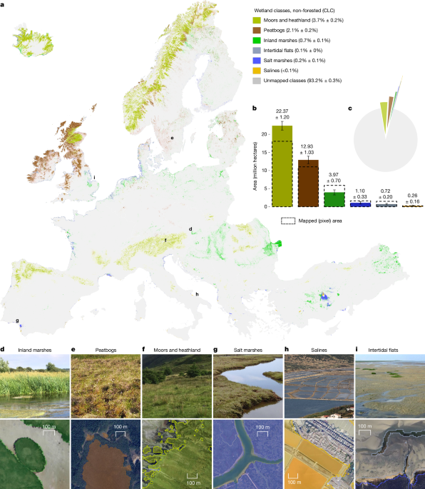
MainWetlands, ecosystems at the land–water interface, are among the planet’s most productive habitats and disproportionate carbon stores4. Although they cover only 5–8% of Earth’s land surface, they hold 20–30% of global soil carbon (2,800–4,300 Gt CO2) and strongly influence long-term climate regulation5. Wetland types arise from gradients in hydrology, geomorphology, climate, soils, salinity, nutrients and vegetation, producing distinct biogeochemical regimes and greenhouse-gas fluxes1. Peatlands, for example, defined by persistent peat accumulation, contain the largest stores6. Yet human activities have driven a 16–23% global loss of inland wetlands since the 1700s, with warming compounding continuing degradation2. Undisturbed wetlands act as carbon sinks, whereas drainage and intensive management convert stocks to emissions6,7.Europe is a hotspot of historical loss: average wetland extent has declined by more than 50% since 1700 and by more than 75% in several countries, mainly through systematic drainage for agriculture and forestry2. In response, the EU NRL (Regulation (EU) 2024/1991) mandates restoring ecosystems not in ‘good condition’8 with targets of 30% by 2030, 60% by 2040 and 90% by 2050 (ref. 3). Article 4 covers terrestrial, coastal and freshwater ecosystems and defines restoration as actions that move systems towards their original condition (for example, rewetting, hydrological reconnection, pollution abatement, native species reintroduction)3. Effective delivery requires measurable, comparable indicators9, yet information on the condition of natural and seminatural wetlands remains limited and inconsistent across countries10.To provide a harmonized, spatially explicit baseline covering priority wetland habitats under Article 4 (Supplementary Table 1), we use the CORINE Land Cover (CLC) framework11 to target Europe’s main natural and seminatural open wetland classes (‘inland marshes’, ‘peatbogs’, ‘salt marshes’, ‘salines’, ‘intertidal flats’ and ‘moors and heathland’), while excluding densely forested wetlands that the CLC framework does not distinguish from other forests. Under present EU/Intergovernmental Panel on Climate Change (IPCC) land-use classifications, drained peat soils managed as cropland or grassland fall under NRL Article 11 and tree-covered organic soils under Article 12 (forestry accounting with limited voluntary rewetting)3; these deeply drained former wetlands (no sustained saturation or hydrophytic vegetation) are therefore outside our scope here to avoid double counting with Article 4, which targets natural and seminatural wetlands.The CLC framework’s standardized definitions align with European carbon assessments1 but its manual interpretation, multiyear update cycle and 25-ha minimum-mapping unit hinder timely detection and bias against small, managed mosaics, propagating errors in distribution and carbon estimates12. Meeting restoration objectives thus requires high-resolution, standardized, regularly updated mapping of wetland extent, type and disturbance. Here we map six open wetland types at 10-m resolution across Europe (2018 epoch) by combining optical and radar satellite data in a scalable machine-learning framework anchored to the CLC framework. The resulting geodataset refines carbon-stock estimates and quantifies anthropogenic impacts at national to subcontinental scales, providing the spatial detail needed to guide Article 4 restoration for 2030 and beyond.European-scale mapping of open wetlandsWe mapped six natural and seminatural open wetland types across large parts of Europe at 10-m resolution with an overall accuracy of 96.6 ± 0.3%, covering an estimated 413,504 ± 17,782 km2, equivalent to 6.8 ± 0.3% of the respective land surface (Fig. 1). This was achieved using an eXtreme Gradient Boosting (XGBoost)13 machine-learning algorithm trained on 101,000 CLC-labelled sample points and applied to a multisensor satellite data cube spanning 2017–2019. The resulting 49-variable predictor set combined optical and radar observations from more than 470,000 Sentinel-1 and Sentinel-2 scenes with auxiliary geospatial layers on topography, climate, biomes and soil across 38 European countries (EEA38; Methods). Cloud-free median composites of key spectral and temporal features were generated and extracted from Google Earth Engine14. To quantify mapping-related uncertainty, we combined the mapped wetland classes with an independent, visually interpreted validation sample to derive sample-based area estimates and associated uncertainty measures (Methods). European-scale wetland areas and map accuracies were estimated directly from the independent stratified reference sample using a design-based estimator. Country-level wetland areas were estimated using a hierarchical framework that combines calibration weighting with empirical-Bayes partial pooling to stabilize estimates in which national sample sizes are limited (Methods). These area estimates, together with their associated 95% confidence intervals reported as ± values, are used in all subsequent analyses.Fig. 1: Map of six main wetland types (natural and seminatural CLC classes) in Europe (EEA38 countries).a, Continental-scale wetland cover mapped in six main classes by machine learning and 10-m resolution satellite imagery for 2018. b,c, Area coverage of wetland types in Europe, with mapped and sample-based area estimates in million hectares (b) and proportion of the total area spanning 38 countries (c). d–i, Examples of individual wetland classes: inland marshes in Hungary (d); peatbogs in Sweden (e); moors and heathland in Austria (f); salt marshes in Spain (g); salines in Italy (h); intertidal flats in the United Kingdom (i). Error bars and ‘±’ values denote 95% confidence intervals, calculated as ±1.96 × standard error from the stratified, area-weighted sample-based estimator. n = 10,975 sample points. Further examples are shown in Supplementary Figs. 1 and 2. Photos: LUCAS 2018 (ref. 31). Basemap imagery © Google/Maxar Technologies.Among Europe’s CLC inland wetland categories (Fig. 1 and Supplementary Fig. 1), the class ‘moors and heathland’ covers the largest area, with 223,662 ± 11,985 km2 (3.7 ± 0.2% of the continent; producer’s accuracy (PA) = 76%; user’s accuracy (UA) = 96%). It also includes, by definition, several Arctic, Alpine and maritime non-wetland habitats. ‘Moors and heathland’ are concentrated in high-latitude regions (for example, Norway, Iceland) or high-altitude zones (the Alps, Scottish Highlands), in which lower temperatures and persistent moisture dampen vegetation growth, evapotranspiration and decomposition. Although differently classified as ‘shrubland’ or ‘wetland’ in land-cover products11,15,16,17, they play an important role in carbon sequestration18. ‘Peatbogs’, stretching 129,325 ± 10,323 km2 (2.1 ± 0.2%; PA = 67%; UA = 92%), are principally found in northern Atlantic areas, in which postglacial landforms and abundant precipitation support peat accumulation and bog development. ‘Inland marshes’, totalling 39,698 ± 6,975 km2 (0.7 ± 0.1%; PA = 90%; UA = 79%), encompass a variety of wetlands with herbaceous vegetation, including fens and transitional mires, often concentrated in river valleys, floodplains, deltas and lakeside areas. Smaller coastal wetlands (‘intertidal flats’, ‘salt marshes’, ‘salines’) occupy 20,819 ± 4,154 km2 (0.3 ± 0.1%) of Europe (Fig. 1 and Supplementary Fig. 2). Within these zones, ‘salt marshes’ (11,023 ± 3,267 km2; 0.2 ± 0.1%; PA = 94%; UA = 75%) are scattered mostly along Atlantic and North Sea coasts, the western and central Mediterranean shores and parts of the Black Sea margin, shaped by salt-tolerant vegetation, sedimentary processes and tidal flow. ‘Intertidal flats’ (7,191 ± 2,007 km2; <1%; PA = 98%; UA = 45%), occurring along the Atlantic, are continually shaped by coastal dynamics, whereas ‘salines’ (2,605 ± 1,619 km2; <0.1%; PA = 81%; UA = 78%), the smallest class, represent both active and formerly exploited salt-evaporation basins.National coverage varies markedly and skews northward: Norway (>100,000 km2) holds the largest extent, followed by the United Kingdom, Iceland, Sweden, Ireland and Finland, a pattern consistent with wet, cool climates and low-relief postglacial terrains that sustain waterlogging, peat formation and long-term carbon storage (Extended Data Fig. 1).Direct cross-dataset comparisons showed overall agreement in wetland extent but are hampered by inconsistent typologies and mapping frameworks19,20,21,22,23,24 (Extended Data Fig. 2, Extended Data Table 1 and Supplementary Figs. 3–6). Calculating the patch-size distribution (contiguous clusters of 10-m cells within a class) shows that European wetlands are fine-grained and highly fragmented, with an estimated 27–33% of wetland area occurring in map-defined patches <25 ha and 7–11% in patches <1 ha (Extended Data Table 2 and Supplementary Fig. 7). Small-patch prevalence is greatest for inland marshes (48.8% <25 ha; 19.8% <1 ha), followed by salt marshes and lowest for intertidal flats (15.2% <25 ha; 5.2% <1 ha), consistent with long-term fragmentation in intensively used landscapes. By contrast, widely used land-cover and wetland products under-represent this class and size diversity: wetlands <25 ha (≈500 × 500 m) and <1 ha (≈100 × 100 m) are commonly missed by coarser inventories.Together, these results show that fine spatial detail is essential to represent wetland extent and heterogeneity across Europe. They also provide the robust spatial basis needed for continental-scale carbon stock estimates, which cannot be consistently derived from coarser-resolution products.Carbon stock estimatesBuilding on this high-resolution wetland extent, we next estimated associated soil carbon stocks across Europe. Carbon stock calculations used sample-based wetland area estimates, with stratified estimates at the European scale and calibrated hierarchical estimates at the country level (Methods). We then applied published ranges of soil organic carbon (SOC) density (Mg C ha−1)1,10 to estimate corresponding carbon stocks for each CLC wetland class in every country (Extended Data Table 3 and Methods). These density ranges synthesize measurements from several studies across Europe sampled over different depth intervals (consistent with the CLC framework), from surface soils (0–10 cm, 0–20/30 cm) to full peat profiles (1–3+ m), depending on wetland type (Supplementary Table 2), capturing depth-integrated variability in soil carbon. Our estimates exclude carbon stocks from drained and forested wetlands. The resulting total wetland carbon storage potential spans 2.8–14.3 Gt C, broadly consistent with earlier estimates (3.2–8.4 Gt C)1,10, while indicating a higher upper bound.At the national level, the respective carbon stocks peak at 3.5 Gt C in the United Kingdom, 2.7 Gt C in Norway and 2.5 Gt C in Sweden, reflecting values at the upper end of our range (Fig. 2). By CLC wetland class, ‘peatbogs’, although covering only about 2% of the study area, store on average 3.3 Gt C (53% of the mean pool) (Fig. 2). ‘Moors and heathland’ account for 1.8 Gt C (29%), whereas ‘inland marshes’, despite limited area, contain 0.9 Gt C (14%), making them the most carbon-dense type in countries such as Turkey, Romania, Hungary and Poland. Notably, large portions of areas mapped as ‘inland marshes’ in the Central European Lowland and the Danube Delta correspond to fen peatlands16.Fig. 2: Carbon storage potential across European (EEA38) countries and (semi)natural CLC wetland classes.a,b, Geometric-mean estimates of potential carbon stocks in total wetlands for 2018, showcasing contributions per type at the country level and across Europe, with ‘±’ values denoting 95% confidence intervals, calculated as ±1.96 × standard error from the stratified, area-weighted sample-based estimator. For each country (and for Europe), the 2018 mean estimate is calculated as the geometric mean of the lower and upper bounds of the total carbon-stock range obtained by aggregating class-specific minimum and maximum stock estimates. c, Cross-country comparison of total carbon storage in wetlands, showing geometric-mean estimates (bars), the corresponding stock ranges (error bars) and type proportions.Owing to high burial rates, coastal wetlands also contribute disproportionately: ‘salt marshes’ cover just 0.2% of the study area yet store 0.3 Gt C (5% of the total pool) and also have low CH4 and N2O emissions25,26. Although ‘tidal flats’ have emerged as notable global carbon sinks27, their European stocks remain poorly quantified28 and their carbon storage potential is not well understood. We therefore highlight the need for targeted in situ measurements of ‘tidal flats’ in Europe. In the absence of such data, both ‘intertidal flats’ and ‘salines’ are excluded from our carbon accounting analyses.Human disturbance patternsAlthough undisturbed wetlands typically act as carbon sinks, human disturbances in wetlands can lead to a shift in their carbon balance, causing a net carbon loss from wetland soil to the atmosphere29. Wetlands located within or near agricultural or urban areas are probably influenced by human activities such as land development, pollution, soil compaction, vegetation removal and drainage30. Consequently, wetlands under agricultural or urban land use are expected to fail to meet the NRL’s ‘good condition‘ thresholds3, given their compromised distribution, structural integrity and characteristic species compositions.To distinguish (semi)natural wetland areas under anthropogenic pressure and characterize wetland condition at the continental scale, we used agricultural and urban land-use classes as proxies for physical, chemical and biological stressors. We intersected the 10-m wetland map with CLC2018 agricultural and urban polygons and computed distance to these features to assign each wetland pixel to a disturbance category (Fig. 3). Wetlands overlapping these land-use classes were classified as ‘most disturbed’, those within 150 m as ‘intermediately disturbed’ and all others as ‘least disturbed’. At the European scale, disturbance-domain areas were obtained using the design-based stratified estimator. At the country scale, disturbance areas were derived by calibrated allocation from the pooled country-level wetland-class totals, with uncertainty propagated by Monte Carlo sampling (Methods).Fig. 3: Anthropogenic land-use disturbances in European (semi)natural CLC wetland classes.a, Anthropogenic disturbances in three disturbance levels. b–e, Examples of disturbed wetlands include converted ‘salt marshes’ near the Doñana National Park, southern Spain (b); ‘peatbogs’ used for pasture near Lough Ree in Ireland (c); ‘moors’ used for agriculture on Gurskøy island, Norway (d); and ‘inland marshes’ converted to cropland in the Danube Delta, Romania (e). f, Share of wetland area in each disturbance class by wetland type. g, EEA38-wide share of wetland area in each disturbance class, derived from sample-based area estimates. The ‘±’ values denote 95% confidence intervals, calculated as ±1.96 × standard error from the stratified, area-weighted sample-based estimator. n = 10,938 sample points. Basemap imagery © Google/Maxar Technologies.Our estimates indicate that 20.4% ± 3.4% of Europe’s wetland area is affected by anthropogenic disturbance, with 13.6% ± 3.0% classified as most disturbed (Fig. 3). Regional patterns indicate that undisturbed wetland areas are predominantly situated in high-altitude and high-latitude regions, such as the Alps, the Scandinavian mountains, the Scottish Highlands and Iceland. These undisturbed areas align with ‘moors and heathland’, confirmed as the least disturbed (87.7% ± 4.0%) CLC wetland class in Europe, probably because of their location in agriculturally unfavourable terrains with difficult access. By contrast, ‘inland marshes’ represent the most disturbed wetland ecosystems, with nearly half of their area classified as most disturbed. This is followed by ‘salt marshes’, in which roughly one-third (about 36%) of the area shows signs of disturbance, and ‘peatbogs’, in which around one-fifth (about 21%) is affected by human activity.Disturbance varies sharply across countries (Extended Data Fig. 3 and Supplementary Table 3). In absolute terms, the United Kingdom (1.35 Mha), Ireland (0.97 Mha), Turkey (0.79 Mha), Romania (0.67 Mha) and France (0.58 Mha) host the largest disturbed extents. However, the relative share of disturbed wetlands differs substantially, ranging from 23.7% in the United Kingdom and 21.6% in Spain to 59.5% in Turkey and 49.7% in Romania. The highest proportional disturbance occurs in Bulgaria (78.8%), Serbia (75.7%), Hungary (71.3%) and Poland (70.9%), despite their smaller absolute areas (<0.4 Mha). By contrast, Iceland (95.4% ± 2.6%), Norway (95.1% ± 1.9%), Sweden (94.0% ± 1.1%) and Finland (93.2% ± 2.4%) retain the highest shares of undisturbed wetlands. At the other end of the gradient, Norway (4.4%), Iceland (5.3%), Finland (5.7%) and Sweden (8.5%) retain the lowest disturbed shares, with most wetland extent remaining intact at northern latitudes. Although disturbed areas in these countries range from about 0.1 to 0.5 Mha, the predominance of undisturbed wetlands may partly reflect the exclusion of deep-drained and forested wetlands from our accounting.Wetland carbon storage lossTo estimate potential carbon storage losses from human disturbance, we applied wetland-specific and disturbance-specific reduction factors (Extended Data Table 4) derived from large-scale differences in measured carbon stocks across disturbance levels and wetland types29 to the baseline carbon stocks described above. We evaluated these factors against approximately 22,000 SOC measurements from the LUCAS 2018 topsoil dataset31 (0–20 cm) across Europe and found that the magnitude of the observed decline is broadly consistent with our reduction factors and generally lies towards their lower bound (Extended Data Fig. 4). This near-surface focus for carbon exchanges is consistent with IPCC guidelines and peatland flux studies, which identify the upper approximately 30 cm as the main aerobic decomposition zone, in which repeated oxygen exposure drives most CO2 emissions, whereas deeper layers (>30 cm) remain largely anoxic and decompose more slowly32,33.For each wetland type and country, the potential carbon storage loss is defined as the difference between the undisturbed baseline and the disturbance-adjusted stock, expressed in CO2-equivalent (CO2-eq) units (Methods). Summed across wetland classes and countries, these estimates indicate a disturbance-associated stock difference observed under 2018 conditions, rather than a realized emission trajectory over a specified time period. Land-use disturbances correspond to potential losses of 0.8–4.9 Gt CO2-eq, equivalent to roughly 10–11% of the mean soil carbon storage pool in European wetlands (Extended Data Table 3). By inheriting the variability of the underlying carbon-density values, these potential loss estimates reflect heterogeneity in topography, peat depth, land use and management. ‘Peatbogs’ show the widest spread and therefore the broadest ranges of potential losses (0.3–3.8 Gt CO2-eq). All estimates represent 2018 conditions and quantify potential carbon storage losses associated with contemporary land-use disturbance, rather than annual greenhouse-gas emission rates, and are restricted to natural and seminatural open wetlands, excluding historically lost wetlands, forested wetlands and heavily drained peatlands34.Our findings reveal the highest potential carbon-storage losses in the United Kingdom, Norway, Sweden and Ireland, reflecting the combination of large wetland extents and substantial disturbance (Fig. 4 and Supplementary Table 4). At the upper end of our estimated ranges, potential losses reach 1,125 Mt CO2-eq in the United Kingdom, 812 Mt CO2-eq in Sweden, 679 Mt CO2-eq in Norway and 553 Mt CO2-eq in Ireland. Across wetland types, potential carbon losses are strongly concentrated in ‘peatbogs’ (0.32–3.78 Gt CO2-eq), reflecting their high carbon densities and disturbed extent. ‘Inland marshes’ contribute 0.32–0.71 Gt CO2-eq, followed by ‘moors and heathland’ (0.13–0.26 Gt CO2-eq) and ‘salt marshes’ (0.07–0.13 Gt CO2-eq). Overall, disturbance-driven carbon vulnerability in Europe is structurally dominated by peatbogs (Fig. 4).Fig. 4: Loss of carbon storage potential in European CLC wetland classes owing to anthropogenic disturbances.a, Geometric (log) mean loss of carbon storage potential owing to disturbances across countries in 2018, with relative country-level contributions by open wetland type. Potential carbon storage loss is estimated relative to an undisturbed baseline (Fig. 2). b, Geometric (log) mean carbon storage potential in wetlands across countries after adjustment for anthropogenic disturbances. c, Estimated range of carbon storage loss in wetlands across countries. d, Estimated range of potential carbon storage loss per wetland type. Floating bars represent the minimum–maximum range derived from variability in the underlying carbon stock measurements, whereas the dashed lines indicate the geometric (log) mean for reference. Estimates represent differences in potential soil carbon stock under the 2018 disturbance state relative to the undisturbed baseline and do not imply a specific temporal rate of carbon loss.Restoration targets across countriesIn line with the ‘good condition’ criteria of the Habitats Directive8, which encompass distribution, structural integrity and characteristic vegetation, we interpreted land-use disturbance in wetlands as a signal of non-compliance and translated it into scenario-based wetland restoration target areas (Methods). At the country level, we define the restoration target as the area of (semi)natural open wetlands under land-use disturbance that may be eligible for restoration under these criteria. These country-level restoration target areas should be interpreted as stylized scenarios, assuming that a fixed share of disturbed seminatural open wetlands is restored to meet the Article 4 percentage targets, rather than as exact legal obligations or implementation plans. For each Article 4 scenario, the restoration area was calculated as the mandated percentage of the estimated disturbed wetland area for each wetland type and country (Fig. 5 and Supplementary Table 5). Disturbed areas were derived from country-level estimates, with uncertainty propagated from the underlying area estimators.Fig. 5: Restoration targets for seminatural wetlands across European (EEA38) countries by 2030.a,b, Country-level restoration targets by 2030 across Europe showing 30% of disturbed wetland area across all types (a) and 30% of the total disturbed ‘peatbogs’ area (shown separately owing to high carbon relevance; carbon stocks can be equally large in fen peatlands included in the class ‘inland marshes’ but this class also includes low-carbon wetlands and is therefore not shown separately) (b). c, Comparison of total disturbed seminatural wetland area and 2030 restoration targets per country with the EEA38 average. Error bars denote 95% intervals from Monte Carlo propagation of the country-level calibrated wetland area estimates and the calibrated disturbance-allocation procedure. n = 5,000 Monte Carlo draws.According to our estimates, 2.66 Mha of wetlands would need to be restored by 2030 across the EEA38, corresponding to an average national target of approximately 70,000 ha. Several countries far exceed this value: the United Kingdom (403,700 ± 99,300 ha), Ireland (290,300 ± 73,600 ha), Turkey (237,500 ± 100,400 ha) and Romania (200,700 ± 68,400 ha) together account for a large share of the total. The United Kingdom’s eligible restoration area is nearly four times that of Germany (105,600 ± 52,200 ha). France (173,900 ± 57,400 ha), Denmark (144,400 ± 51,200 ha) and Norway (141,700 ± 33,500 ha) also stand well above the regional average, whereas Sweden (99,400 ± 35,200 ha), Poland (104,300 ± 56,200 ha) and Hungary (89,300 ± 49,100 ha) cluster closer to the mean despite contrasting land areas.In northern Europe, restoration targets are strongly influenced by peatbog distribution. Peatbog-specific targets reach 234,000 ± 71,300 ha in the United Kingdom and 256,900 ± 64,900 ha in Ireland, with Sweden (91,600 ± 35,100 ha) and Norway (38,000 ± 14,600 ha) also showing substantial peatland components. By contrast, Turkey and Romania, in which peatbog extent is limited, show large overall targets (237,500 and 200,700 ha, respectively), driven mainly by inland marsh systems.Taken together, these country-level patterns show that restoration demand reflects the distribution of seminatural wetland types and their disturbance within each country, underscoring the need for harmonized, spatially detailed wetland datasets to enable robust cross-border comparison of restoration commitments.Comparison with existing productsTo place our estimates in context, we next compared our 10-m wetland map with existing continental-scale wetland products. Our cross-product assessment revealed that many existing wetland maps and reporting systems are limited by incompatible typologies. Broader class definitions are often misaligned with specific policy aims such as the NRL. For example, some inventories group forested wetlands and drained peat soils into broad classes, whereas others (for example, tidal-only products) exclude inland types altogether. Compiled layers often mix heterogeneous national legends, so class definitions can drift across borders. Coarser pixels or large minimum-mapping units tend to systematically omit or merge small wetland patches, biasing area metrics. Time adds another axis of inconsistency: many compilations integrate legacy geodata from different decades, so ‘extent’ may reflect historical distributions and can retain wetlands that are now degraded or lost without stating this explicitly. When explicitly distinguished from present wetland extent rather than conflated with it, however, such legacy layers can still be valuable for locating degraded or lost wetlands now under agriculture, particularly drained peat soils relevant to NRL Article 11. A further constraint of existing products is the limited quantification of uncertainty: accuracies, when reported, are often presented without confidence intervals or an explicit sampling design, restricting their use in planning, model-based assessments and applications requiring uncertainty propagation. By contrast, our 10-m European wetland map applies a single, continent-wide methodology grounded in standardized wetland definitions and resolves sub-hectare structure, reducing omission of small patches. We report confidence-bounded accuracies and sample-based area estimates and the workflow is reproducible and updatable for change assessment, providing a comparable baseline for restoration planning across Europe. Combined with explicit legal targets, this framework supports operational comparison and tracking of restoration pathways under the EU NRL.To anchor the magnitude of our restoration scenario estimates in existing policy contexts, we compared our 2030 target areas for all wetlands against national pledges and found that some countries are well on track to meet their restoration objectives (Extended Data Fig. 5 and Supplementary Table 5). These comparisons use national total areas only and do not assume spatial overlap between our estimated restoration targets and pledged sites, as national definitions of areas allocated to restoration may differ from the wetland categories used here. Among these frontrunners, Denmark’s 2030 wetland-specific pledge is in near one-to-one agreement with our 2030 estimate (Δ ≈ 3%, within uncertainty). In the United Kingdom, peat-only commitments lie near the upper bound of our peatbog-only 2030 estimate, exceeding the mean by about 31% and falling only roughly 1% below the upper 95% confidence limit35. Ireland’s confirmed projects correspond to about 47% of our peatbog-only 2030 estimate and about 42% of our all-wetlands 2030 estimate, with further sites under preparation36. Germany’s emissions-based (≥5 Mt CO2-eq year−1 from peat soils by 2030) milestone corresponds to about 89% of our 2030 estimate, reflecting a substantial rewetting pipeline already in motion37. Continued joint wetland restoration efforts along the Danube floodplain38,39 in Austria, Hungary, Slovenia, Croatia, Serbia, Romania and Bulgaria could contribute towards meeting each country’s 2030 NRL obligations. Romania’s long-term objective exceeds our 2040 estimate (+17%), whereas Hungary’s 2030 pledge represents only about 40% of our estimate, implying restoration potential three to five times higher than the present commitment, consistent with previous assessments38. Finland stands out: its 2030 goal of 60,000 ha (ref. 40) equals about 175% of our 2030 estimate and about 87% of our 2040 figure, probably reflecting broader definitions (that is, forested peatlands, including bog woodland) beyond our ‘peatbogs’ class. However, restoration of forested wetlands typically requires tree removal and is therefore strictly capped under the NRL, limiting how such areas can be counted towards NRL targets. Nevertheless, the success of restoration is measured not only in hectares restored but also in the protection and retention of soil carbon in disturbed wetlands.European wetlands and global carbonTo discuss restoration in a broader climatic context, we compared the magnitude of potential soil carbon loss associated with land-use disturbance in Europe’s wetlands with realized or observed wetland carbon losses elsewhere. Our estimates are grounded in continent-scale LUCAS Soil observations and indicate a potential loss of 0.84–4.87 Gt CO2-eq, relative to a baseline estimate without land-use disturbance. This magnitude is comparable with cumulative European peatland CO2 emissions reported over recent decades41. However, substantial uncertainty remains about the timescales over which these carbon losses have occurred or may continue, reflecting a central limitation: Europe lacks continent-scale, temporally resolved monitoring of wetland carbon stock change. For comparison, wetlands in the conterminous United States experienced a realized carbon loss of 1.06 Pg C between 2011 and 2016 (ref. 29), equivalent to approximately 3.9 Gt CO2-eq, largely associated with anthropogenic disturbance. Tropical peatland disturbance regimes that include fire have released on the order of 0.8–1.0 Gt CO2-eq over even shorter periods, as during Indonesia’s 2015 fire season6. These examples illustrate that carbon stocks of comparable magnitude can be mobilized within only a few years under sustained pressure. Although restoration often slows or halts further emissions42, it does not replenish depleted carbon stocks or may do so only over much longer timescales43,44. Even full implementation of present restoration targets would therefore not automatically restore carbon already lost from previously disturbed European wetlands. In the absence of harmonized, repeatedly updated inventories of wetland soil carbon across Europe, restoration of disturbed seminatural wetlands is thus both a mitigation strategy and a precautionary measure to prevent further, potentially irreversible, depletion of Europe’s remaining wetland carbon stocks.Limitations and implementation pathwaysWe note several limitations. Typology and boundaries remain imperfect: the CLC class ‘moors and heathland’ intermixes with dry heath in Mediterranean regions, inflating that class, whereas boreal open peatlands (for example, aapa mires) are under-represented in ‘peatbogs’, in which seasonal wetness and woody cover blur separation from ‘inland marshes’. Coastal optical effects can also produce false positives in ‘salines’, in which algal blooms and green water resemble evaporative pans despite contextual screening.Carbon-stock estimates span wide ranges because depth-resolved SOC measurements are sparse, spatially clustered and rarely capture land-use and management effects at depth. Regional variation in carbon densities within classes is likely but further subdivision beyond standardized CLC types would reduce cross-country comparability.Country-level area estimation with hierarchical pooling provides a practical compromise between continent-wide summaries and direct country-domain estimation. Because validation support within individual countries is sparse for some wetland types, and especially for disturbance-specific subdomains, direct country-level estimates can be unstable. A nationally stratified validation design with adequate support for every wetland type and disturbance category in every country would require substantially larger and more costly reference-data collection. Our approach therefore preserves the continental probability-sampling basis while stabilizing sparse country-level estimates through hierarchical pooling towards regional mean compositions. Unlike the Europe-wide design-based estimates, country-level estimates are model-based and their 95% intervals are posterior credible intervals.Even with explicit restoration area targets to 2030, implementation is constrained by logistical, political and financial factors (for example, limited funding, land-use conflicts)45, and the law’s reach is uneven: non-EU partners and candidates participate only voluntarily, whereas the main wetland holders outside the EU (for example, Norway, United Kingdom, Turkey) are not bound by EU rules or supported by the Common Agricultural Policy (CAP). Although the reformed CAP allocates resources to environmental measures, wetland-specific criteria are limited and alignment with the NRL remains weak46. Even in some member states (for example, Lithuania), CAP-linked financing for wetland restoration (GAEC 2) was unavailable before 2025, constraining early implementation. With National Restoration Plans due by 2026, the window for demonstrable progress is narrow, raising the risk that rapid delivery gives priority to area over ecological quality. Even so, the 2030 target may serve as a catalyst, mobilizing institutions, aligning finance and setting a credible trajectory towards extensive wetland restoration by 2040 and beyond.ConclusionWetlands occupy only a small fraction of Europe’s land surface. Our results show that seminatural open wetlands are rare, highly fragmented, heavily modified and important for carbon storage and thus for the global carbon budget. Disturbance is concentrated in inland, carbon-rich systems; restoration needs are unevenly distributed among countries; and many wetlands occur in small patches embedded in Europe’s mosaic landscapes, reflecting centuries of land conversion. Viewed through the lens of the EU NRL, our blueprint shows how harmonized, pixel-scale satellite observations can be translated into restoration policy insights across countries. Until truly continental or global field campaigns can routinely characterize wetland condition and carbon stocks, such large-scale, remotely sensed proxies will remain central to supporting wetland restoration and conservation pledges. In the context of historic wetland loss, aligning legal commitments with ecological understanding and high-resolution, data-driven observation offers a rare opportunity to move from a legacy of loss to an era of targeted restoration, in Europe and globally.MethodsOptical and radar imageryWe used Google Earth Engine14 for the systematic extraction and processing of remote sensing data (Supplementary Fig. 8). For optical data, we used Sentinel-2 (ref. 47) multispectral imagery at 10-m resolution in the visible and near-infrared bands (B2, B3, B4, B8) and 20 m in the shortwave-infrared bands (B11, B12). Sensor-provided quality bands were used to mask clouds and cirrus. From these bands, we derived spectral indices including the normalized difference vegetation index48,$${\rm{NDVI}}=\frac{{\rm{B}}8-{\rm{B}}4}{{\rm{B}}8+{\rm{B}}4},$$and a modified normalized difference water index49,$${\rm{M}}{\rm{N}}{\rm{D}}{\rm{W}}{\rm{I}}=\frac{{\rm{B}}3-{\rm{B}}11}{{\rm{B}}3+{\rm{B}}11},$$as well as a grey-level co-occurrence matrix (GLCM) contrast texture from the near-infrared band (B8) using a 2-pixel window.For radar data, we used C-band Sentinel-1 (ref. 50) synthetic aperture radar imagery at 10-m resolution in VV and VH polarizations, together with the local incidence angle. From these, we derived the VV/VH backscatter ratio (ratio = VV/VH) and its temporal statistics. To provide further thermal context, we also included Landsat-8 (ref. 51) thermal bands, using the provided quality information to remove clouds and cloud shadows.For each sensor and band, we aggregated all cloud-free observations between 2017 and 2019 into monthly median composites. From these monthly stacks, we derived per-pixel temporal statistics (multiyear median, standard deviation and maximum), so that for each band b we obtained$${\tilde{x}}_{b}={{\rm{median}}}_{t}({M}_{b,t}),\,{\sigma }_{b}={{\rm{sd}}}_{t}({M}_{b,t}),\,{x}_{b}^{\text{max}}=\mathop{\text{max}}\limits_{t}({M}_{b,t}),$$in which Mb,t is the monthly median in month t. This yielded, per 10-m pixel, a multisensor predictor image stack summarizing central tendency and intra-annual variability in optical and radar signals.Ancillary dataAs well as optical and radar imagery, we incorporated several ancillary variables. Land-surface temperature was derived from a MODIS daily land-surface temperature product52, using the mean daytime temperature over 2000–2020 (1-km resolution, resampled to 10 m). Total precipitation was obtained from a global atmospheric reanalysis (ERA5)53 using the 2000–2020 mean of daily total precipitation (native resolution approximately 27 km, resampled to 10 m) to provide a long-term hydroclimatic baseline. Topography was represented by the EU-DEM v1.1 (ref. 54) (25-m resolution), from which we computed the slope using a terrain operator; both elevation and slope were included as predictors. We further derived a distance-to-coast layer as the Euclidean distance to the nearest coastline (truncated at 5 km), capturing coastal–inland gradients relevant for salt-influenced wetlands. Following a preliminary soil analysis based on the European Soil Database v2.0 (ref. 55), we included categorical layers for Food and Agriculture Organization of the United Nations (FAO) soil units and parent materials (for example, dystric histosols organic parent materials), as well as terrestrial biomes from the RESOLVE Ecoregions dataset56. These categorical maps were represented as indicator variables (one-hot encodings) for use in the machine-learning model. In total, the resulting feature stack comprised 49 predictor variables per 10-m pixel, spanning spectral, radar, thermal, topographic, climatic, edaphic and biome controls.Mosaic creationOur workflow combines cloud-based preprocessing with high-performance local computing for mosaic creation. All primary predictors (Sentinel-1/Sentinel-2 and Landsat-8 bands, spectral indices, GLCM texture and temporal statistics) and ancillary variables (climate, topography, distance to coast, soils and biomes) were first computed as 10-m, cloud-free composites and long-term summaries within Google Earth Engine. These multiband images were then exported as tiled GeoTIFFs. The European study area (EEA38) was partitioned into country polygons and further subdivided into a regular 5-km grid, aligned with the corresponding local UTM zone to ensure equal-area representation. For each 5-km grid cell, we assembled all predictors into a single multiband mosaic at 10-m resolution, producing local feature stacks as multiband GeoTIFFs in local UTM coordinates, suitable for supervised learning.Training dataWe used the CLC2018 dataset11, covering all 27 EU member states together with extra European Environment Agency (EEA) countries (Andorra, Albania, Bosnia and Herzegovina, Switzerland, Iceland, Liechtenstein, Montenegro, North Macedonia, Norway, Serbia, Turkey and the United Kingdom), hereafter referred to as the EEA38. Throughout, ‘Europe’ and ‘the continent’ refer to this reporting extent. CLC is the most comprehensive continental-scale dataset for wetland types but its minimum-mapping unit of 25 ha omits many small wetlands and introduces uncertainty around land-cover boundaries. Such noisy labels are problematic for convolutional neural networks trained on high-resolution satellite imagery57,58,59. By contrast, pixel-based approaches that use point labels, and are less sensitive to polygon boundaries, have shown strong performance when trained on coarse or noisy annotations60.To construct a supervised training dataset from CLC2018, we selected 101,000 training sample points. Each training location was required to be at least 100 m from CLC class boundaries, reducing label noise from neighbouring land-cover types. We defined seven target wetland classes (inland marshes, peatbogs, salt marshes, salines, intertidal flats, moors and heathland and surface water) based on their corresponding CLC classes. For each wetland class c, we drew nc = 5,000 training sample points, giving a total of$${N}_{{\rm{wet}}}=\mathop{\sum }\limits_{c=1}^{7}{n}_{c}=7\times \mathrm{5,000}=\mathrm{35,000}$$wetland training locations. To represent non-wetland land cover, we drew training sample points from 30 diverse non-wetland and non-water CLC classes, with 2,000 sample points per class, and extra background locations to capture further variability, yielding in total Nbackground = 66,000 training sample points. The full training set thus comprised Ntotal = Nwet + Nbackground = 35,000 + 66,000 = 101,000 training sample points, of which 35,000 represented target wetland classes and 66,000 represented various background (non-wetland and non-water) classes. This stratified design imposed equal sampling effort across wetland classes (5,000 training sample points per class) while also drawing a large and diverse set of background points from many non-wetland land-cover types. At each of the 101,000 training sample locations, we extracted the selected image features (multisensor satellite composites and ancillary layers) using Google Earth Engine14.Model selection and optimizationFor our wetland type classification task, we selected the XGBoost13,61 model because of its efficiency and stability for multiclass classification with noisy labels13. Let (xi, yi) denote training sample i, with feature vector xi and class label yi ∈ {1,…, K}. XGBoost learns an additive ensemble of regression trees$${F}^{(M)}({\bf{x}})=\mathop{\sum }\limits_{m=1}^{M}{f}_{m}({\bf{x}}),\,{f}_{m}\in {\mathcal{F}},$$in which each fm is a decision tree and M is the number of boosting rounds. At each iteration m, the model is updated as$${F}^{(m)}({\bf{x}})={F}^{(m-1)}({\bf{x}})+\eta \,{f}_{m}({\bf{x}}),$$in which η ∈ (0, 1] is the learning rate. The ensemble is trained by minimizing a regularized objective$${\mathcal{L}}=\sum _{i}{\ell }({y}_{i},{F}^{(M)}({{\bf{x}}}_{i}))+\mathop{\sum }\limits_{m=1}^{M}\Omega ({f}_{m}),$$in which ℓ(·) is a multiclass loss (softmax) and Ω(fm) penalizes model complexity (for example, tree depth, number of leaves), which helps control overfitting and improve generalization62. Because the coarse CLC labels introduce label noise, some xiyi are mislabelled. In gradient boosting, instance weights are implicitly updated by means of the gradient of the loss$${g}_{i}^{(m)}=\frac{\partial {\ell }({y}_{i},{F}^{(m-1)}({{\bf{x}}}_{i}))}{\partial F},$$so that trees fm focus on poorly predicted training points while the regularization term Ω(fm) and learning rate η prevent overfitting to noisy labels. In practice, this means that persistently inconsistent or mislabelled points contribute less to the final decision function, which mitigates the effects of label noise on the CLC-based training set.We tuned the XGBoost hyperparameters using random search63 with fivefold cross-validation on the training data. For each candidate hyperparameter vector θj, we computed a cross-validated loss,$$\hat{{\mathcal{L}}}({{\boldsymbol{\theta }}}_{j})=\frac{1}{K}\mathop{\sum }\limits_{k=1}^{K}{{\mathcal{L}}}^{(k)}({{\boldsymbol{\theta }}}_{j}),$$with K = 5 folds and negative mean squared error as the optimization criterion, and retained the configuration with the lowest \(\hat{{\mathcal{L}}}({{\boldsymbol{\theta }}}_{j})\) across 25 candidates (125 fits in total). Cross-validation averages over different training–validation splits, reducing sensitivity to both sampling variability and label noise in the validation folds. The final model used GPU-accelerated boosting with tuned values for the learning rate η = 0.03, maximum tree depth = 9, number of trees M = 1,207, minimum loss reduction (γ) and tree growth policy (depthwise).After predicting wetland classes at 10-m resolution, we applied a 3 × 3 median (mode) filter to the class map to remove isolated speckle and smooth class boundaries, replacing each pixel label by the most frequent class within its 3 × 3 neighbourhood64.Validation dataWe constructed a validation set drawn independently of the training data and not used in model fitting using stratified random sampling with disproportionate allocation, with a minimum of nc = 500 validation sample points for each target wetland class and a planned total of Nval ≈ 15,000 validation locations across all strata (Supplementary Table 6). All non-target strata (non-wetland and non-water CLC classes) were merged into a single background stratum. Stratum areas were derived by intersecting CLC2018 polygons with the 10-m European Forest Type 2018 dataset65, excluding forested regions from the target classes. Within each stratum, we then generated validation sample locations at least 10 m away from all training sample points to ensure spatial independence. Of the planned roughly 15,000 locations, 3,691 could not be placed: the placement algorithm (maximum five attempts per point) could not find positions satisfying the ≥10-m criterion, with the shortfall concentrated in the geometrically narrow salines stratum (208 of 500 planned points generated). A further 326 fell outside the mapped image extent and were removed and eight were excluded during final reference-label quality control because no reliable land-cover label could be assigned, giving Nval = 10,975 sample points.Each validation sample point was visually interpreted on-screen by an expert using high-resolution Google satellite imagery, following the CLC illustrated nomenclature guidelines66, which provide class descriptions, surface-pattern diagrams and example photos to support consistent labelling. Uncertain or ambiguous points were jointly reviewed by two more interpreters until consensus was reached. As contextual information, we consulted the Global Lakes and Wetlands Database v2 (ref. 15) (for broader wetland system type) and the 10 m Water and Wetness 2018 dataset67 (for local patterns of permanent and temporary water and wetness; Supplementary Fig. 9). These ancillary datasets informed interpretation only; final reference labels were assigned solely by expert visual assessment. The sample point retained its original sampling stratum and associated inclusion probability.Europe-wide area and accuracy estimationAt the European scale, wetland area and map accuracy were estimated directly from the independent continental validation sample Nval = 10,975 using design-based stratified estimation. Area estimation followed a stratified estimator using sampling strata defined by collapsed CLC classes (Supplementary Table 6), consistent with standard practice when reporting classes differ from sampling strata68. Let h = 1,…, H index strata with total area Ah and sample size nh. For reference class k, the within-stratum proportion is$${\hat{p}}_{{hk}}=\frac{1}{{n}_{h}}\sum _{i\in h}I({y}_{i}=k),$$in which I(·) is an indicator function and yi the reference label. The stratified estimator of class area is$${\hat{A}}_{k}=\sum _{h}{A}_{h}{\hat{p}}_{{hk}}.$$Under stratified random sampling with finite population correction, the variance is$${\rm{Var}}({\hat{A}}_{k})=\sum _{h}{A}_{h}^{2}\left(1-\frac{{n}_{h}}{{N}_{h}}\right)\frac{{s}_{{hk}}^{2}}{{n}_{h}},\,{s}_{{hk}}^{2}=\frac{{n}_{h}}{{n}_{h}-1}{\hat{p}}_{{hk}}(1-{\hat{p}}_{{hk}}),$$in which Nh = Ah/a is the population size in pixels and a = 100 m2 is the pixel area. Standard errors were \({\rm{SE}}({\hat{A}}_{k})=\sqrt{{\rm{Var}}({\hat{A}}_{k})}\) and 95% confidence intervals were \({\hat{A}}_{k}\pm 1.96{\rm{SE}}({\hat{A}}_{k})\). Estimated areas of the population error matrix (Supplementary Tables 7 and 8) were computed analogously for reference class r and mapped class c:$${\hat{A}}_{{cr}}=\sum _{h}{A}_{h}{\hat{p}}_{{hcr}},\,{\hat{p}}_{{hcr}}=\frac{1}{{n}_{h}}\sum _{i\in h}I({m}_{i}=c,{y}_{i}=r),$$in which mi is the mapped label and yi is the reference label. The overall accuracy was$${\rm{OA}}=\frac{\sum _{k}{\hat{A}}_{{kk}}}{\sum _{c}\sum _{r}{\hat{A}}_{{cr}}},$$with producer’s and user’s accuracies$${{\rm{PA}}}_{k}=\frac{{\hat{A}}_{{kk}}}{\sum _{c}{\hat{A}}_{{ck}}},\,{{\rm{UA}}}_{k}=\frac{{\hat{A}}_{{kk}}}{\sum _{r}{\hat{A}}_{{kr}}}.$$To characterize wetland fragmentation from the mapped patch structure, map-defined patch-size bins were derived from contiguous clusters of 10-m cells within each class. The wetland area in each bin was then estimated using the same stratified-design-based indicator estimator as for class-area estimation, with cumulative categories such as <25 ha estimated directly.Country-level wetland area estimationBecause validation sample sizes for individual wetland classes varied substantially among countries (Supplementary Table 9), direct country-domain estimation alone was often too unstable for reliable reporting and country-level wetland areas were therefore estimated using a calibrated country-level estimator with hierarchical pooling built on the continental stratified probability sample. The domain-estimation motivation follows standard survey-sampling logic for sparse domains69, whereas the implemented estimator combines calibration weighting70,71 with empirical-Bayes compositional pooling72,73,74. Let h index the continental validation strata and d the reporting countries. To preserve the continental sampling basis, initial expansion weights were defined as$${w}_{h}^{(0)}=\frac{{A}_{h}}{{n}_{h}},$$in which Ah is the known total area of stratum h in the analysis frame and nh is the number of validation sample points in that stratum. To align this continental sample with country-level reporting, these base weights were then calibrated by generalized raking, implemented through iterative proportional fitting, so that the weighted sample matched both the known country frame totals Ad and the known continental stratum totals Ah (refs. 70,71). In this setting, calibration estimation refers to the adjustment of design-based expansion weights using known auxiliary totals, thereby linking the continental probability sample to the country reporting domains. This calibration step assumes that, after adjusting to known country-frame and stratum-area totals, the calibrated pseudo-counts are conditionally representative of each country’s true class composition. After calibration, weights were normalized within country and normalized weighted class pseudo-counts were computed for each wetland class k as$${\tilde{n}}_{d,k}=\sum _{i\in {s}_{d}}{w}_{{di}}^{{\rm{norm}}}I(\,{y}_{i}=k),$$in which sd denotes sampled units in country d, \({w}_{{di}}^{{\rm{norm}}}\) the normalized calibrated weight and I(·) an indicator for the final reference class. To stabilize country-specific class compositions when these weighted counts were sparse, countries were assigned to fixed macro-regions and region-level mean class compositions were estimated from pooled weighted country counts. We then used a two-level hierarchical empirical-Bayes Dirichlet formulation, in which each country-level class-composition vector πd was modelled relative to the corresponding macro-regional mean composition μr (refs. 72,73,74). In this hierarchy, country-level compositions are pooled to a shared regional mean for all countries belonging to the same macro-region, with the degree of shrinkage controlled by κ:$${\pi }_{d}|{\mathop{n}\limits^{ \sim }}_{d}\approx {\rm{Dirichlet}}(\kappa {\mu }_{r}+{\mathop{n}\limits^{ \sim }}_{d}),$$in which \({\mathop{n}\limits^{ \sim }}_{d}\) is the vector of normalized weighted country reference pseudo-counts, μr the corresponding macro-regional mean composition for region r and κ a global shrinkage parameter selected by empirical-Bayes grid search to maximize the Dirichlet-multinomial marginal log-likelihood72,73,74. This hierarchical formulation preserves positivity and unit-sum constraints and stabilizes weak country estimates by shrinking them towards macro-regional mean compositions, while allowing countries with more informative weighted counts to remain closer to their own observed class composition72,73. This formulation assumes that countries within each macro-region share broadly similar wetland class compositions (Supplementary Table 9). Posterior draws of πd were scaled by the known country frame area Ad to obtain country-level class area draws, \({A}_{d,k}^{(s)}={A}_{d}{\pi }_{d,k}^{(s)}\). Country-level wetland areas were summarized by posterior means and 95% posterior credible intervals.As a model check, for all 15 countries with effective sample size neff ≥ 200 (spanning all five macro-regions), direct calibration-only estimates of total wetland area fell within the 95% posterior credible interval in all cases (mean absolute relative difference 3.2%); for countries with fewer sample points, wider credible intervals reflect appropriately increased uncertainty. For these data-rich countries, low pooling fractions (κ/(κ + neff) < 0.12) ensure that country-level calibration data dominate the posterior; the hierarchical structure mainly serves to regularize estimates for countries with sparse validation support, for which direct estimation would be unstable. At the macro-regional level, the aggregate of pooled posterior means across all countries in each of the five regions fell within the 95% posterior credible interval in all cases, with deviations of less than 2.2% from the corresponding direct calibration aggregate.Wetland disturbance area estimationAnthropogenic disturbance was defined by intersecting the wetland map with agricultural and urban classes from CLC2018. Wetlands overlapping these classes were classified as most disturbed, those within 150 m of them as intermediately disturbed and all others as least disturbed. Disturbance labels were assigned after sampling and treated as post-stratification reporting domains. Europe-wide areas (EEA38) for disturbance levels and wetland class–disturbance combinations were estimated within the wetland domain using the same stratified indicator estimator described above. At the country level, further post-stratification by disturbance further reduced effective sample sizes within individual wetland classes. Country-level disturbance subdomain areas were therefore estimated by calibrated allocation from the pooled country-level wetland class totals. Let Ac,k denote the pooled country-level area for wetland class k and \({\hat{A}}_{k,d}^{{\rm{EEA}}38}\) the European design-based area for class k and disturbance level d. The EEA38 disturbance composition within class was defined as$${q}_{k,d}^{{\rm{EEA}}38}=\frac{{\hat{A}}_{k,d}^{{\rm{EEA}}38}}{\sum _{d}{\hat{A}}_{k,d}^{{\rm{EEA}}38}}.$$Mapped within-country disturbance shares \({p}_{c,k,d}^{{\rm{map}}}\) were used as auxiliary information to form initial allocations$${A}_{c,k,d}^{(0)}={A}_{c,k}{p}_{c,k,d}^{{\rm{map}}}.$$These were calibrated within class to satisfy$$\sum _{d}{\tilde{A}}_{c,k,d}={A}_{c,k},\,\sum _{c}{\tilde{A}}_{c,k,d}=\left(\sum _{c}{A}_{c,k}\right){q}_{k,d}^{{\rm{EEA}}38}.$$Calibration was implemented by means of iterative proportional fitting. Uncertainty was propagated by Monte Carlo sampling of pooled country totals and Europe-scale disturbance estimates, with calibration repeated for each draw.Carbon storage estimationSample-based wetland area estimates formed the basis for carbon-stock calculations. At the European scale, stratified class-area estimates derived from the stratified validation sample were used. At the country scale, calibrated hierarchical estimates provided country-level wetland areas. Carbon-density ranges (Mg C ha−1) were compiled from a meta-analysis of 34 studies1 and harmonized to CORINE wetland classes (Extended Data Table 3). These ranges encompass variability in vegetation, soils, peat depth and land use1. Although CORINE distinguishes shallow and deep peat, no explicit depth threshold was imposed, as the density ranges used already integrate this variation. For wetland class k, carbon stock (Gt C) was calculated as$${C}_{k}^{v}=\frac{{A}_{k}{\rho }_{k}^{v}}{{10}^{9}},$$in which Ak denotes the sample-based area estimate and \({\rho }_{k}^{v}\) the minimum, maximum or geometric-mean carbon density. The geometric mean was computed as$$\bar{\rho }=\exp \left(\frac{{\mathrm{ln}\rho }_{\text{min},k}+{\mathrm{ln}\rho }_{\text{max},k}}{2}\right),$$motivated by the log-normal behaviour of SOC observed in LUCAS topsoil data (Supplementary Fig. 10). Country-level carbon stocks were obtained by summing across wetland classes.Adjustment for human disturbancesDisturbance-specific wetland areas were estimated directly. At the European scale, disturbance-domain areas were obtained using the design-based stratified estimator described above. At the country scale, disturbance areas were derived by calibrated allocation from the pooled country-level wetland-class totals, with uncertainty propagated by Monte Carlo sampling of posterior area draws. Carbon densities were adjusted as$${\rho }_{k,d}^{v}=(1-{R}_{k,d}){\rho }_{k}^{v},$$in which Rk,d denotes the class-specific reduction factor (Extended Data Table 4). For peatbogs, reductions of 0%, 30% and 50% were assumed for the least, intermediate and most disturbed categories; for other wetland types, reductions of 0%, 20% and 25% were applied. These values were evaluated against LUCAS SOC observations and were conservative relative to observed depletion patterns (Extended Data Fig. 4). Disturbance-adjusted carbon stocks were calculated as$${C}_{k,d}^{v}=\frac{{A}_{k,d}{\rho }_{k,d}^{v}}{{10}^{9}},$$with baseline stocks$${C}_{k}^{v,{\rm{base}}}=\frac{{A}_{k}{\rho }_{k}^{v}}{{10}^{9}}.$$Potential carbon stock loss was defined as$$\Delta {C}_{k}^{v}={C}_{k}^{v,{\rm{base}}}-\sum _{d}{C}_{k,d}^{v},$$and converted to CO2 equivalents using the molar mass ratio 44/12.Determining restoration targetsIn line with the EU NRL targets under Article 4, we derived scenario-based restoration target areas for (semi)natural open European wetlands failing the ‘good condition’ criteria owing to anthropogenic disturbance using country-level, sample-based disturbance-area estimates. For each country c, disturbed wetland area was defined as the sum of intermediately and most disturbed categories across wetland classes,$${\hat{A}}_{c,{\rm{dist}}}=\sum _{k}({\hat{A}}_{c,k,1}+{\hat{A}}_{c,k,2}),$$and classwise disturbed area as \({\hat{A}}_{c,k,{\rm{dist}}}={\hat{A}}_{c,k,1}+{\hat{A}}_{c,k,2}\). Restoration targets were then computed as fixed fractions of disturbed area,$${T}_{c}^{2030}=0.30\,{\hat{A}}_{c,{\rm{dist}}},\,{T}_{c}^{2040}=0.60\,{\hat{A}}_{c,{\rm{dist}}},$$with classwise targets defined analogously (\({T}_{c,k}^{2030}=0.30\,{\hat{A}}_{c,k,{\rm{dist}}}\); \({T}_{c,k}^{2040}=0.60\,{\hat{A}}_{c,k,{\rm{dist}}}\)). Given the high carbon density of peatbogs, we also reported peatbog-specific targets based on \({\hat{A}}_{c,{\rm{peat}},{\rm{dist}}}\). Uncertainty was propagated by applying the same target fractions to each Monte Carlo draw of \({\hat{A}}_{c,{\rm{dist}}}\) and summarizing targets using 95% empirical intervals (Fig. 5 and Supplementary Tables 4 and 5). Finally, we benchmarked the estimated 2030 targets against published national wetland and peatland restoration commitments for the 15 countries with the largest disturbed wetland area, compiled from official policy documents (Extended Data Fig. 5 and Supplementary Table 5).All analyses were implemented in Python.
Highly fragmented European wetlands with uneven restoration needs - Nature
Satellite imagery and machine learning used for the mapping of six seminatural open wetland types and land-use disturbance in European countries shows that wetlands are highly fragmented and have uneven restoration needs.
11,048 words~50 min read