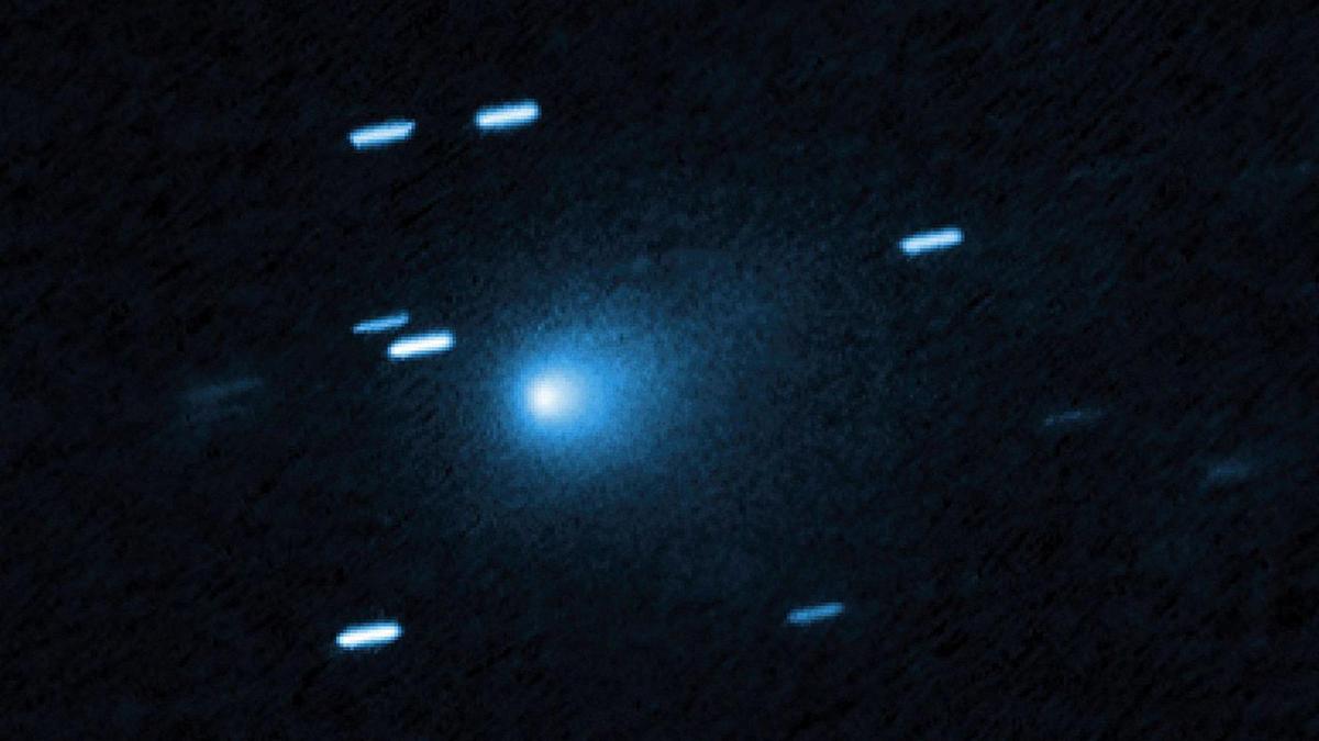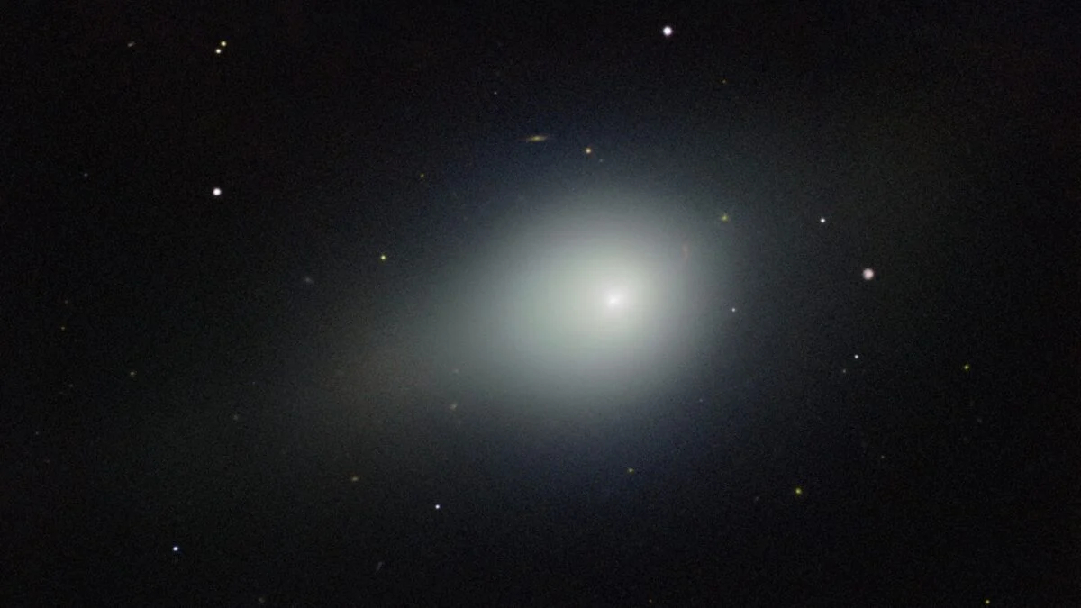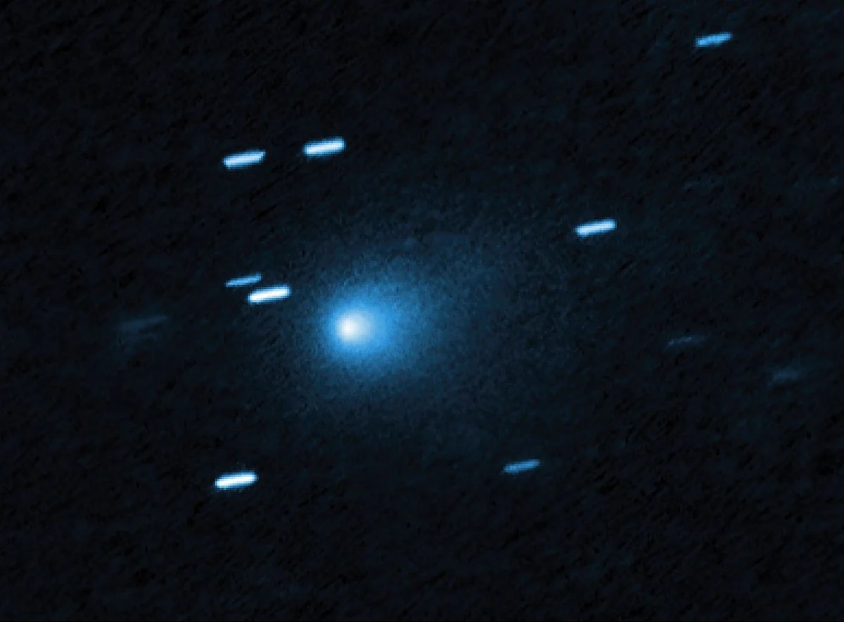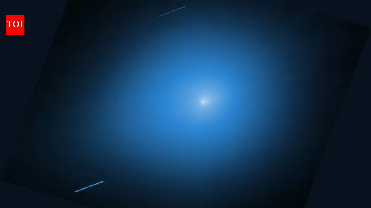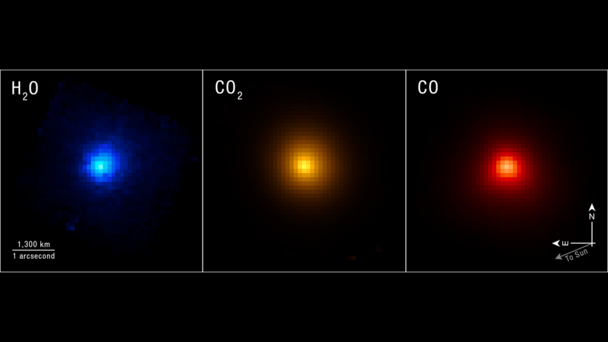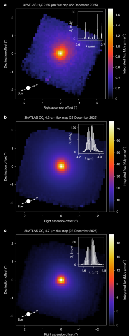
Main3I/ATLAS is the third confirmed interstellar object to pass through our inner Solar System4. It showed surprisingly high gas production rates around perihelion, which have enabled detailed spectroscopic investigations3,5,6,7. However, its exact time and place of origin, and the history of its path through the Galaxy, remain highly uncertain8,9,10. A broad range of ages (3–11) Gyr was deduced based on its high velocity, but tracing the orbital trajectory back more than about 10 Myr is difficult owing to unpredictable (chaotic) gravitational interactions within the inhomogeneous Galactic environment11. Isotopic ratio measurements provide invaluable insights into the physical and chemical conditions where 3I/ATLAS formed12: the D/H ratio is sensitive to the temperature and radiation environment13, and the 12C/13C ratio reveals the degree of heavy-element enrichment (metallicity), which helps constrain the location (in space and time) of its natal interstellar gas cloud14.JWST and ALMA observationsWe obtained infrared spectral imagery of 3I/ATLAS using the James Webb Space Telescope (JWST) during the outbound leg of its 2025 perihelion passage. We simultaneously targeted emission lines from gas-phase water (H2O), carbon dioxide (CO2) and carbon monoxide (CO) (major isotopologues), in addition to their respective (deuterium (D) and 13C bearing) minor isotopologues, allowing the derivation of precise isotopic ratios. The 2.7-μm H2O fundamental rovibrational bands were observed on 22 December 2025, with a subsequent, deeper integration covering H2O (hot bands), HDO, CO2, 13CO2, CO and 13CO between 3.6 μm and 5.0 μm on 23 December 2025 (see Methods for details). A summary of the observed molecular bands is given in Extended Data Table 1. For the purpose of measuring the coma expansion velocity, complementary, ground-based submillimetre-wave observations of 3I/ATLAS’s CO and HCN emission were obtained using the Atacama Compact Array (ACA; a subsystem of the Atacama Large Millimeter/submillimeter Array (ALMA)) on 22 December 2025 (Methods). 3I/ATLAS was at a heliocentric distance rH ≈ 2.4 au for all observations.Multiple spectral lines from each of the major isotopologues were detected across the entirety of the Near-Infrared Spectrograph (NIRSpec) field of view, confirming the presence of a spatially extended gas coma, with a peak intensity at the assumed position of the nucleus (the pseudo-nucleus). The image cubes for the major isotopologues were baseline-subtracted using a polynomial fit to the surrounding continuum regions in each pixel, then spectrally integrated to produce the molecular emission maps shown in Fig. 1. Spatially integrated spectra (within a d = 3.6″-diameter circular aperture centred on the pseudo-nucleus) are shown for all the species of interest in Fig. 2.Fig. 1: Spectrally integrated line flux maps for 3I/ATLAS observed using JWST NIRSpec.a–c, H2O at 2.7 μm (a), CO2 at 4.3 μm (b) and CO at 4.7 μm (c). Image axes are aligned with the equatorial (right ascension/declination) grid. Molecular emission has been isolated by subtracting a polynomial fit to the adjacent continuum. Spatial coordinates are with respect to the brightest pixel in each map (the pseudo-nucleus). Insets: the continuum-subtracted spectra within the image integration wavelength range, spatially integrated within a 3″-diameter circular aperture centred on the pseudo-nucleus (corresponding to 3,900 km at the 1.8 au distance of the comet from the telescope). The bottom-left corner shows the direction of the (sky-projected) comet–Sun (S) and nucleus velocity (v) vectors. Sλ is the spectrally integrated emission line flux; λ is the wavelength.Fig. 2: Observed NIRSpec molecular spectra of 3I/ATLAS.a–f, Spectra have been integrated within a d = 3.6″-diameter circular aperture centred on the pseudo-nucleus. Similarly spatially integrated, best-fitting spectral models are overlaid, with (observation minus model) residuals in the bottom panels. As shown by the grey filled regions in a, the strong CO (v = 1–0) lines were subtracted (sub.) before fitting, to reduce spectral contamination when fitting H2O. The grey region in d indicates wavelengths excluded (masked) from the fitting owing to potential contamination by an unidentified feature around 4.42 μm. In f, the regions surrounding the stronger CO lines (shown in grey) were masked during 13CO fitting, to avoid contamination by the CO model residuals, and to allow improved fitting of the higher total angular momentum (J) CO lines, some of which overlap 13CO. For d and f, fifth-order baseline fits are shown; see Extended Data Fig. 3 for the ensemble of baselines used in deriving our final range of plausible 12C/13C values for these species.Gas production rates (Q), rotational temperatures (Trot) and isotopic ratios were derived by modelling the observed infrared emission lines as a function of sky-projected nucleocentric distance (ρ) using the Planetary Spectrum Generator (PSG)15 (Methods). The resulting Qρ curves for CO2 and CO (Extended Data Fig. 1) reach a clear asymptote (‘terminal’ Q value) at ρ ≈ 0.3″ (about 400 km), indicating a lack of significant gas production for these species at larger radii, consistent with the majority of their outgassing arising directly from the nucleus. H2O shows a significant increase in Qρ between ρ ≈ 0.3″ and ρ ≈ 1.7″ (about 500–2,200 km), consistent with a contribution to the H2O gas production from icy grain sublimation in the coma; uniformity of the HDO/H2O ratio with radius (within the errors) implies similar gas release mechanisms for both H2O and HDO.Terminal gas production rates (Qt) were calculated for each species from the average of the Qρ values in the five outermost annuli shown in Extended Data Fig. 1, and are given in Extended Data Table 1. From these production rates, we find the following mixing ratios (and 1σ statistical uncertainties) for the main coma gas constituents within the JWST field of view: CO2/H2O = 1.08 ± 0.03; CO/H2O = 2.40 ± 0.07; CO/CO2 = 2.24 ± 0.01. Since the earlier 6 August 2025 JWST observations5 (obtained at rH = 3.32 au inbound), the coma CO2/H2O ratio has fallen by a factor of approximately 7, and the CO/H2O and CO/CO2 ratios have increased by factors of approximately 1.4 and approximately 10, respectively. This corresponds to a transition from a CO2-dominated to a CO-dominated coma during the object’s passage past the Sun (bracketing a likely H2O-dominated phase around perihelion6), indicating a remarkable temporal evolution of the relative outgassing rates for these coma gases.From the simultaneously-measured Qt(HDO) and Qt(H2O) values (Methods), we derive a D/H mixing ratio for water of (0.98 ± 0.06)%. Spectral baseline definition is more challenging for 13CO2 and 13CO than HDO, so for those species we report the results considering an ensemble of best-fitting Qt values across a range of plausible baseline models (the associated data are given in Extended Data Tables 2 and 3), resulting in 12C/13C = 141–191 for CO2 and 123–172 for CO. These ranges include the (additive) statistical 12C/13C uncertainties of 2% for CO2 and 8% for CO, and should therefore be interpreted as the range of plausible fit parameters for each molecule.Interpreting the isotopic ratiosThe D/H and 12C/13C ratios for 3I/ATLAS are both extremely unusual among previously observed comets and other Solar System objects (Fig. 3). Although previous measurements of the 12CO2/13CO2 ratio have been obtained in only two comets (67P and C/2017 K2), the 12C/13C ratio of the broader reservoir of volatile carbon in the Solar System (including other cometary gases), is well characterized. Observations of methane (CH4) in Jupiter, Saturn and Neptune, CO2 on Mars and Venus, CH4 ice on Eris and Makemake, as well as carbonates (and insoluble organic matter) in meteorites, and CN and C2 in comets, all show remarkably similar 12C/13C ratios, consistent with terrestrial sedimentary rocks (12C/13C = 89.4), to within a few per cent, whereas the solar ratio is 93.5 ± 0.7 (ref. 16). The elevated 12C/13C ratios in 3I/ATLAS are therefore completely distinct from other materials measured in the Solar System, thus highlighting a non-local origin. The unusual isotopic ratios are supported by the recent findings of Salazar Manzano et al. 17 and Opitom et al.18, who also found increased D/H and 12C/13C ratios for 3I/ATLAS based on their respective ALMA and Very Large Telescope observations (see Supplementary Discussion for further details).Fig. 3: Galactic and Solar System isotopic ratios.a,b, Observed isotopic ratio in the coma of 3I/ATLAS compared with Galactic and Solar System observations for D/H (a) and 12C/13C (b). Different symbols are used for the different categories of planetary and astronomical objects. Data are from the compilation of ref. 12, with additional D/H values for 12P/Pons-Brooks36, V883 Ori (gas phase37), and IRAS 20126+4104, HOPS370 and L1527 (ice phase38,39). D/H data are for H2O unless otherwise specified. The ‘disks HCN’ data represent the mean and range of observed D/H values across five protoplanetary disks. ‘MYSOs’ data are the mean and range for massive young stellar objects. For 12C/13C, the range of plausible fit results (including 1σ statistical errors) is given for 3I/ATLAS. The meteoritic ‘XCO3’ and ‘IOM’ data are the mean values (and ranges) for carbonates and insoluble organic matter, respectively, in carbonaceous chondrites40,41,42. We also plot TW Hya and HD 163296 CO isotopic ratios43,44, mean protostellar ice CO and CO2 values45, protostellar CO gas (mean and range)46, interstellar medium (ISM) CO2 ice (mean and range)47, ISM HCO+ isotopic ratios for two Galactocentric distances (rG)21, rG = 14 kpc CN data19, super-Jupiter exoplanet CO data48, and M-dwarf GJ745 data49. Error bars are 1σ unless otherwise specified.Even outside the Solar System, measurements of 12C/13C > 100 are rare, although such high ratios are predicted (and occasionally observed) in the outer parts of the Galaxy14,19,20,21. The primary source of carbon in our Galaxy is from nucleosynthesis in the envelopes of asymptotic giant branch stars, with additional, minor contributions from novae and supernovae14,22,23. Over their lifetimes, intermediate-mass asymptotic giant branch stars return material to the interstellar medium with increasingly elevated elemental 13C abundances, owing to the conversion of 12C to 13C during hot bottom burning (via the CN cycle). Consequently, the cycle of star formation and death leads to increasing metallicity and decreasing 12C/13C ratios in the interstellar medium as a function of Galactic age14. In particular regions where non-equilibrium chemistry can prevail, molecular 12C/13C ratios are subject to further modulation, as a result of isotope-selective photodissociation and low-temperature chemical kinetics12,24,25,26. These processes can either deplete or enhance the 12C/13C ratios in hydrocarbons and nitriles, yet their impact on the 12C/13C ratio in CO—the main carbon reservoir in dense interstellar clouds—is typically small. The relative insensitivity of interstellar CO and CO2 ice to isotopic fractionation processes at low temperatures contributes to the relative consistency of 12C/13C ratios across the Solar System. Consequently, the 12C/13C ratio in primitive planetary (and cometary) materials, including CO, CO2 and their chemical derivatives, is thought to be close to the interstellar elemental value at the time of formation of the host star.The elemental abundances observed in 3I/ATLAS place strict requirements on the chemical profile of its originating star system, which, combined with dynamical constraints from the object’s Galactic orbit (deduced from its inbound velocity vector), result in a set of criteria that help isolate its origin in space and time—see Supplementary Discussion (and Supplementary Table 1) for further details.In a sample of 63 nearby solar-type stars, 12C/13C ratios were measured in the range 71–105 (ref. 27). On the basis of their ages, which span about 0–9 Gyr, a relatively rapid onset of 13C enrichment was inferred, during the first 4 Gyr of our Galaxy’s evolution, as a consequence of 13C production in novae28. The resulting steep 12C/13C curve at early times in their model with 3–8 M⊙ white-dwarf nova progenitors (Supplementary Fig. 1) constrains the isotopic age of 3I/ATLAS to the range 11–12 Gyr, assuming an origin in the nearby Galactic disk. For comparison, the secondary 12C/13C peak at metallicity log10[Fe/H] = −0.5 in Fig. 19 of ref. 14 (thick-disk model), corresponds to a similar estimated age of about 11 Gyr.Uncertainties in the modelled 12C/13C ratios as a function of time are significant owing to incomplete knowledge of the stellar initial mass function, star formation rates as a function of time (and Galactocentric radius), interstellar gas infall and outflow rates, and stellar nucleosynthetic yields. A conclusive age estimate for 3I/ATLAS is further complicated by the interstellar 12C/13C gradient as a function of Galactocentric distance19,21,29 (Supplementary Discussion). Ultimately, 12C/13C ratios within the range of plausible 12C/13C fit values for 3I/ATLAS can be most readily explained as a result of temporal evolution of the interstellar 12C/13C ratio, with a possible additional contribution from the Galactic radial 12C/13C gradient.The D/H ratio for water in 3I/ATLAS demonstrates a surprisingly high D enrichment compared with other (icy and non-icy) Solar System bodies and protostars within the Galaxy (Fig. 3a). The value of (0.98 ± 0.06)% lies 15σ above the mean D/H of 0.029% in Solar System comets (where σ is the combined standard deviation of the data), and 10σ above the mean water D/H of 0.1% found in the total sample of high- and low-mass protostars. Within the Solar System, only Venus’s atmosphere has a higher D/H, which results from mass-dependent atmospheric escape over the planet’s lifetime30. By contrast, the deuteration of H2O ice in Solar System comets is theorized to occur primarily in the interstellar and pre-stellar phases, where H2O is rapidly synthesized on the surfaces of dust grains at very low temperatures (≲30 K)31,32. Reference 13 showed that water deuteration occurs efficiently in star-forming regions as long as the dust temperatures remain below 20–30 K, whereas increased ultraviolet radiation fields and cosmic-ray ionization rates actually accelerate the reactions responsible for deuterating H2O; a high D/H ratio of approximately 1% is achieved in the presence of a cosmic-ray flux ≳10 times the local Galactic value. Such enhanced-ionization conditions would be expected in the vicinity of the lower-metallicity region of early, intense star formation indicated by the high 12C/13C ratio and high abundances of C and O (α-elements) in 3I/ATLAS. Several other properties of low-metallicity environments are theorized to accelerate the deuteration of H2O ice, as summarized in Supplementary Discussion.A systematic difference is observed between the HDO/H2O ratios in nearby protostellar envelopes and those found in Solar System comets (Fig. 3a). Although the number statistics are small for clustered and isolated protostars, the lower D/H ratios in clustered environments can be attributed to higher temperatures and a shorter, low-temperature protostellar collapse phase, that leads to inhibited D enrichment13. The D/H ratio in Solar System comets may have been further reduced by thermochemical reprocessing of H2O in the disk, as a consequence of radial mixing or sublimation and re-freezing, resulting in the incorporation of re-equilibrated H2O (with a lower D/H) back into the ice, thus lowering the bulk D/H ratio33. The exceptionally high D/H ratio measured in 3I/ATLAS therefore implies H2O ice formation at very cold temperatures in an irradiated interstellar or protostellar environment, followed by a lack of significant, high-temperature reprocessing of its water in the disk. Although molecular ice and planetesimal formation is expected to be less efficient in reduced metallicity environments34,35, the HDO-rich composition of 3I/ATLAS proves that the cold, ice-rich conditions required for cometary accretion can still be maintained in less metal-rich (13C depleted) disks.ConclusionJWST observations of the interstellar comet 3I/ATLAS have revealed exceptionally high D/H and 12C/13C ratios in its coma. The observed elemental and isotopic abundance profile places strong constraints on the temperature and star-formation history of its originating environment. To obtain D/H = 0.98%, the bulk of 3I/ATLAS’s H2O ice must have formed at temperatures ≲30 K, with minimal contamination from water (re-)processed at higher temperatures. Its old, 13C-poor natal environment was most likely embedded in a strongly irradiated, interstellar cloud at relatively low metallicity, but enriched in C and O (and to lesser extents, N and S) in the aftermath of an intense period of massive star formation. Its distant origin in space and time makes 3I/ATLAS a valuable tool for Galactic archaeology, highlighting the potential for interstellar object studies to help reveal the broader physical and chemical history of the Milky Way.MethodsJWST observationsObservations of 3I/ATLAS were performed using the JWST NIRSpec integral field unit (IFU)50, as part of programme ID 5094. The G235H dispersive element was used for a single 642-s exposure starting at 03:36 UT on 22 December 2025, covering wavelengths λ = 1.7–3.2 μm, followed by 5 × 700 s exposures with the G395H disperser starting at 08:07 UT on 23 December 2025, covering λ = 2.9–5.3 μm. The resulting 30 × 30 array of spectra have a resolving power Rλ = λ/Δλ ≈ 2,700 and a pixel size of 0.1″, which is approximately the same as the full-width at half-maximum (FWHM) of the JWST point-spread function at 3 μm.3I/ATLAS was acquired and tracked in the IFU using Jet Propulsion Laboratory (JPL) Horizons ephemeris solution #42. During observations, the object was 1.80 au from the telescope, at rH = 2.37–2.42 au, with a (Sun–target–observer) phase angle of 22.7–21.6°. Each exposure was divided across 4 dither positions, spatially separated (in the approximate shape of a square) with offsets of approximately 0.2″ from the (central) targeted position. The data were reduced using the JWST Calibration Pipeline software version v1.20.251 using the JWST Calibration Reference Data System context file 1464. The multiple dithers for each exposure were shifted and combined in the rest frame of the comet during image processing, thus allowing detector artefacts and cosmic-ray events to be identified and removed. For each 3I/ATLAS exposure, a set of sky background exposures with matching exposure time, disperser and dither settings was obtained, offset by 300″ from the science target, along the horizontal axis of the IFU aperture. Unfortunately, two of the five background exposures for G395H failed owing to guide-star acquisition issues, and were not available at the time of writing this manuscript. These failed background exposures were re-observed on 25 April 2026, at a sky position matching their originally intended positions. Inspection of the available background exposures showed no evidence for significant emission from any background (for example, interstellar) infrared sources or zodiacal light, so the final science data cubes were reduced without background subtraction to maximize the signal-to-noise ratio (SNR).After centring on the comet, the individual exposures were combined and rebinned onto a common spatial–spectral coordinate system using the three-dimensional drizzle algorithm included as part of the JWST pipeline’s cube_build task52. The resulting image cube spatial dimensions were approximately 3.7″ × 3.5″ for G235H and approximately 4.4″ × 4.0″ for G395H. The absolute flux calibration accuracy of the final data cubes is expected to be 3% (https://jwst-docs.stsci.edu/jwst-calibration-status/nirspec-calibration-status/nirspec-ifu-calibration-status).To produce spectrally integrated emission maps, the observed data cubes in the vicinity of each emission band were first continuum subtracted (pixel by pixel), using polynomial fits to the spectral baseline regions surrounding the detected emission lines. For H2O, a 7th-order polynomial was used (fitted between 2.55 μm and 2.90 μm); for CO2, 1st order was used (fitted between 4.188 μm and 4.500 μm, with the CO2 ν3 band masked between 4.20 μm and 4.44 μm); for CO, 4th order was used (fitted between 4.50 μm and 4.85 μm). Spectral line emission was excluded from the continuum fits using an iterative sigma-clipping algorithm with a rejection threshold 2.8 times the residual root mean square (RMS) noise level. The detected line emission was then spectrally integrated to produce the maps in Fig. 1. Although the SNR per pixel was too low to allow useful mapping of the minor isotopologues (HDO and 13CO), significant emission from these species is detected in larger extraction apertures (Fig. 2).AstrometryTo guarantee the acquisition of 3I/ATLAS within the small (3″ × 3″) NIRSpec IFU field of view, while allowing for the 0.2″ dither offsets and 0.1″ telescope blind pointing accuracy, we had to ensure an ephemeris accuracy better than ±1.2″ (at 3σ confidence). To reach such a high accuracy, we performed astrometric measurements of 3I/ATLAS in the weeks leading up to our JWST observations using images contributed by observers at various professional telescope facilities, located at sites with good seeing conditions (see ‘Acknowledgements’ for further details). These included the Canada-France-Hawai’i Telescope, the Lowell Discovery Telescope, the Apache Point Observatory, the Southern Astrophysical Research Telescope, the Las Cumbres Observatory, and the University of Hawai’i 2.2 m telescope. Good seeing was essential to resolve the inner coma and the pseudo-nucleus with the greatest possible precision, ensuring a positional measurement as close as possible to the actual location of the cometary nucleus.In the presence of asymmetric outgassing, the inner coma is often distorted in an antisolar direction, and most common astrometric centroiding procedures tend to become biased away from the nucleus and towards the tail. This issue was mitigated using the comet-specific, zero-aperture extrapolation method53,54. Astrometry was reported to the Minor Planet Center, ensuring that it would be available by the time of scheduling and properly included in the solution posted on the JPL Horizons database.Spectral modellingGas production rates (Q) and rotational temperatures (Trot), were derived as a function of distance from the nucleus for H2O, CO2 and CO, using optimal estimation routines as part of the PSG15 (based on synthetic fluorescence models described by ref. 55). To take advantage of the spatial information in our dataset, our modelling strategy followed a similar ‘Q curve’ formalism to that used by previous JWST cometary studies5,56. Pixels close to the nucleus are affected by pont spread function (PSF)-related flux losses and (for stronger lines) opacity effects, which are difficult to accurately model. We therefore derived gas production rates as a function of ρ within successive 0.2″-wide annuli, centred on the brightest (pseudo-nucleus) pixel. Assuming uniform, isotropic gas production with a constant outflow velocity (vout), the Q value converges to an asymptote, or terminal Q value (Qt), at a characteristic ρ value, at which point the unmodelled flux losses are negligible and Qt then represents the total molecular production rate within the field of view. To avoid contamination of these results by noisier pixels at the IFU edges, the Q curves were computed up to ρ = 1.8″, corresponding to the 3.6″-diameter circular integration apertures used in Fig. 2. The gas outflow velocity was set to 0.310 km s−1 for H2O and CO2, and 0.345 km s−1 for CO, based on contemporaneous observations of the spectrally resolved HCN and CO line shapes, using the ALMA ACA (see ‘ALMA observations’). Molecular photolysis rates appropriate for the active Sun were incorporated from ref. 57. The spectral resolution for each NIRSpec grating (as a function of wavelength) was taken from the dispersion curves available at https://jwst-docs.stsci.edu.Statistical 1σ parameter uncertainties were derived from the diagonal elements of the fit covariance matrix, scaled according to the square root of the reduced chi-square (\({\chi }_{{\rm{R}}}^{2}\)) to ensure the baseline noise level was realistically accounted for. For all species apart from CO2, the spectral baseline shape (with contributions due to scattered sunlight and thermal emission from the coma dust and nucleus, combined in some cases with instrumental artefacts) was determined by fitting a polynomial function simultaneously with the gas emission lines. This way, statistical uncertainties in the baseline shape are propagated into the final uncertainties on each Q value. For CO2, the inaccurate model fit to some of the higher total angular momentum (J) CO2 lines (possibly owing to the presence of multiple Trot components or non-local thermodynamic equilibrium (LTE) effects) results in the baseline fit becoming skewed in the direction of the fit residuals. Therefore, before performing the CO2 Q-curve analysis, it was necessary to subtract a fitted linear baseline from these data pixel by pixel (with the CO2 + 13CO2 line-containing region masked between 4.20 μm and 4.44 μm). Owing to the high CO2 line-to-continuum ratio (about 200), uncertainties in the baseline placement for this species have negligible impact on its retrieved production rate.When fitting individual isotopologues, PSG reports total production rates summed over all isotopologues assuming terrestrial isotopic abundance ratios. Therefore, to obtain individual isotopologue Q values, it was necessary to multiply the PSG results by the terrestrial abundance fractions, given at https://hitran.org/docs/iso-meta/.The H2O band at 2.7 μm (in the G235H setting) contains multiple, high-SNR, spectrally resolved rovibrational lines of the ortho (o)- and para (p)-H2O spin states (with H-atom spins parallel versus antiparallel, respectively), so this band was used to determine Trot(H2O) and the H2O ortho-to-para ratio (OPR)—key parameters for reliably measuring Q(H2O) from the weaker, more blended 4.5–5.1-μm H2O hot bands that were observed simultaneously with HDO in the G395H setting. We modelled o- and p-H2O simultaneously, but as separate species, allowing Q(o-H2O), Q(p-H2O) and Trot to vary as free parameters, and with a seventh-order polynomial baseline. An example of the spectral fit quality is shown in Extended Data Fig. 4.The terminal (asymptotic) p-H2O production rate is Qt = (3.79 ± 0.02) × 1026 s−1, and for o-H2O, Qt = (1.04 ± 0.01) × 1027 s−1, leading to OPR = 2.74 ± 0.03, with a total (terminal) water production rate Qt(H2O) = (1.42 ± 0.01) × 1027 s−1, summed over the ortho and para contributions. Owing to the large o- and p-H2O emission line strengths compared with the continuum around 2.7 μm, these results are not significantly dependent on the choice of baseline polynomial order. The 3I/ATLAS OPR is consistent with a spin temperature of Tspin ≈ 35 K (ref. 58). The fact that the associated H2O rotational temperature of 14.5 ± 0.1 K is considerably smaller than the spin temperature implies that the H2O OPR is not being dictated by Trot. Furthermore, constancy of the OPR as a function of radius indicates that it is not being significantly altered within the coma, and instead reflects conditions associated with the release of water from the nucleus.The H2O hot bands around 5 μm contained insufficient unblended lines for a reliable Trot and OPR retrieval, but as they were observed simultaneously with HDO, the hot-band lines were used to derive Qt(H2O) for direct comparison with Qt(HDO). For the H2O hot band (and HDO), the OPR was fixed at 2.74 and the rotational temperature for each annulus (Trot(ρ)) was held fixed according to the Trot(ρ) values previously derived from the H2O 2.7 μm band. Many of the H2O hot-band lines in our data are blended with lines from CO, CN and OCS; therefore, to derive Q(H2O), we focused on the 4.5–4.7 μm region, which contains 3 of the stronger, unblended H2O lines (Fig. 2a). Before fitting the H2O spectrum in each annulus, we subtracted the interloping CO lines, using a set of independent Gaussian fits, to facilitate identification of the spectral baseline. The spectral regions within the boundaries of each subtracted CO line (Fig. 2a) were further masked to prevent any remaining CO line residuals from biasing the fit. The resulting Qρ(H2O) curve is shown in Extended Data Fig. 1a. Taking the average of the outer 5 annuli gives Qt(H2O) = (1.64 ± 0.05) × 1027 s−1, which is 15% larger than the value obtained from the G235H setting on the previous day, indicative of moderate temporal evolution in 3I/ATLAS’s activity.Four individual rovibrational lines of HDO were clearly detected, as part of the ν1 band between λ = 3.55 μm and λ = 3.85 μm (Fig. 2b). No evidence for other significant emission lines, including OH prompt emission, could be identified in this spectral region. A possible weak line of H2CO could be present at 3.689 μm, just to the red of the 3.692 μm HDO line, but H2CO contamination of the HDO signal is expected to be negligible, considering that the expected (stronger) H2CO lines between 3.58 μm and 3.61 μm are not readily apparent in our data. Owing to a relatively complex continuum shape in this region, a seventh-order polynomial was required to obtain a good fit to the baseline. The HDO rotational temperature within a d = 3″ circular aperture (16 ± 3 K) was found to be consistent with that of H2O at 2.7 μm, which justifies the application of the Trot(ρ)(H2O; 2.7 μm) values during the HDO fitting. Taking the average of the outer 5 annuli of the Q-curve (Extended Data Fig. 1a) results in Qt(HDO) = (3.20 ± 0.19) × 1025 s−1. This corresponds to Qt(HDO)/Qt(H2O) = (1.95 ± 0.13) × 10−2, or D/H = (0.98 ± 0.06)% (taking into account the number of hydrogen atoms in H2O).To determine Qρ(CO2) and Trot(ρ)(CO2), the continuum-subtracted NIRSpec data cube was simultaneously fit for CO2 and 13CO2 components in the range 4.15–4.50 μm. These values were then held fixed to derive Qρ(13CO2) using the non-continuum-subtracted cube (confined within the spectral range 4.34–4.50 μm), but this time including a variable polynomial baseline in the PSG retrieval. Continuum definition is non-trivial in the vicinity of the 13CO2 band owing to the presence of a relatively broad, unidentified spectral feature on the long-wavelength side of the 13CO2 P-branch (around 4.42 μm), combined with the close proximity of the main CO2 band on the short-wavelength side of the Q-branch, for which the high-J lines are not accurately modelled. We therefore investigated the effects of continuum uncertainty on Qt(13CO2) by generating an ensemble of Q-curve fits, each with a different polynomial baseline order (between 1 and 5). Owing to potential contamination of the 13CO2 P-branch by the aforementioned unidentified spectral feature, we also performed a separate ensemble of fits, masking the region between λ = 4.380 μm and λ = 4.445 μm (to exclude the 13CO2 P-branch as well as the unidentified feature). The resulting range of fitted baselines is shown in Extended Data Fig. 3a. The corresponding Qt(13CO2) values (and associated 12C/13C ratios) for each of the fitted baselines are shown in Extended Data Table 2, along with the reduced χ2 values (\({\chi }_{{\rm{R}}}^{2}\)) for the (model minus fit) residuals. From the best-fitting Qt(CO2) value of (1.76 ± 0.01) × 1027 s−1 combined with the range of possible Qt(13CO2) values, we derive Qt(CO2)/Qt(13CO2) = 141–191 (including the 1σ statistical error margins on each retrieved measurement).The region between λ = 4.5 μm and λ = 5.1 μm contains the strong v = 1–0 band of CO, in addition to a blend of 13CO, H2O, CN and OCS emission features. Retrieving the 12CO/13CO ratio therefore requires careful modelling of all these features. All gases were modelled as parent species apart from CN, for which the parent scale length was taken from ref. 59. We performed a Q-curve analysis for CO by fitting the production rates for all species as a function of ρ, in addition to retrieving Trot(ρ)(CO) (Extended Data Figs. 1c and 5), with a fifth-order polynomial baseline included in the PSG fit. The resulting terminal production rate was Qt(CO) = (3.94 ± 0.01) × 1027 s−1. The fit to the CO v = 1–0 band is very good apart from in the highest-J CO lines, some of which are blended with lines of 13CO (Fig. 2e). Therefore, to retrieve Qρ(13CO), we focused on the λ = 4.71–5.05 μm region (which contains 15 individual lines of 13CO), with the poorly fitting higher-J CO lines masked out so that those regions did not influence the fit (Fig. 2f). We performed the Q-curve analysis for 13CO by fixing the rotational temperatures according to the previously retrieved Trot(ρ)(CO) curve, with polynomial baseline orders between 1 and 5; in each case, the polynomial coefficients were optimized during fitting so that their uncertainties propagated into the final error estimates on Qρ(13CO). The resulting range of fitted baselines is shown in Extended Data Fig. 3b. Owing to the weakness of the lines, the 13CO signal became too noisy towards the edge of the field of view, so the last two annuli were omitted from the 13CO Q-curve analysis (Extended Data Fig. 1c). The best-fitting Qt(13CO) value and associated 12C/13C ratio and \({\chi }_{{\rm{R}}}^{2}\) for each baseline order is given in Extended Data Table 3, corresponding to a range of 12CO/13CO values between 123 and 172 (including 1σ statistical error margins).Taking the average of the last 5 points in the Q curves for CN and OCS, from our fits to the λ = 4.5–5.1 μm region, the resulting Qt(CN) and Qt(OCS) values for each baseline order are given in Extended Data Table 3. Averaged over the set of 5 different baseline orders, we derive Qt(CN) = (3.10 ± 0.6) × 1024 s−1 and Qt(OCS) = (4.70 ± 0.49) × 1024 s−1, where the errors are the average statistical uncertainties combined in quadrature with the standard deviations of the respective Qt values (across the 5 different baseline orders). Qt(CN) should be considered a strict lower limit because CN is produced in the comae of Solar System comets with a radial scale length of approximately 3 × 10⁴ km (ref. 60), so the majority of its production is expected to occur outside of the NIRSpec field of view.The measured OCS/CO2 production rate ratio is (0.27 ± 0.03)%. This is significantly less than the values of 0.6–0.9% found in comet 67P/Churyumov–Gerasimenko61, and may indicate a relatively low elemental S/O value for the 3I/ATLAS originating system.ALMA observationsSubmillimetre interferometric observations of comet 3I/ATLAS were obtained with the ACA subcomponent of ALMA as part of ALMA project 2025.A.00004.S. The observations were conducted in nominal Band 7 weather conditions on 22 December 2025 between 07:32 and 08:36 UT, using 11 × 7-m antennas, with a median zenith precipitable water vapour column of 0.33 mm. The Band 7 receiver was configured to simultaneously observe the CO J = 3–2 line at 345,795.990 MHz at a spectral resolution of 122 kHz and the HCN J = 4–3 line at 354,505.477 MHz at a spectral resolution of 61 kHz. The position and radial velocity of the object were tracked using JPL Horizons solution #44. The interferometric data were flagged and calibrated in the Common Astronomy Software Applications (CASA) package62 using standard scripts supplied by the Joint ALMA Observatory. The interferometric point-spread function was then deconvolved from the spectral image data using the CASA tclean Hogböm algorithm with natural weighting, using a mask size equal to the primary beam FWHM and stopping at a threshold of twice the RMS noise. The resulting (two-dimensional Gaussian) beam FWHM was 5.08″ × 3.37″ for CO and 4.91″ × 3.28″ for HCN.The molecular spectra were extracted from the CO and HCN integrated emission peak position, then subjected to modelling using the SUBLIME radiative transfer code63, to derive the gas outflow velocities (vout). The latest theoretical state-to-state collisional rates were used for H2O–CO (ref. 64) and H2O–CN (ref. 65), with photolysis rates for the active Sun57 and solar pumping rates from refs. 63,66. For the HCN J = 4–3 line, hyperfine components were included as described by ref. 67. Our calculations assumed Qt(H2O) = 1.7 × 1027 s−1 and a kinetic temperature Tkin = 40 K (based on Trot = 40.3 ± 0.3 K retrieved from our JWST CO data within a d = 3″ circular aperture). Ideally, collisions with CO and CO2 should also be considered in the SUBLIME molecular excitation calculation, but in reality, the retrieved outflow velocities are not affected by the assumed collision rates. Because the gas coma of 3I/ATLAS is larger than the maximum recoverable scale for the ACA (approximately 19″), interferometric flux losses were modelled by applying a constant flux loss factor of 0.75 for the central beam, which was derived by comparing the peak flux of our model CO image before and after processing it using the CASA simobserve task.Assuming a spherically symmetric coma, the best-fitting SUBLIME models gave vout(CO) = 0.345 ± 0.010 km s−1, Q(CO) = (2.64 ± 0.01) × 1027 s−1, vout(HCN) = 0.276 ± 0.015 km s−1 and Q(HCN) = (6.75 ± 0.54) × 1024 s−1 (Extended Data Fig. 2). These gas outflow velocities are smaller than the values of about 0.5 km s−1 typically found in comets at similar heliocentric distances, which can be explained as a result of outgassing driven by a species with a higher molecular weight than H2O (ref. 3). This is consistent with the high CO2/H2O and CO/H2O abundances (greater than unity) measured in 3I/ATLAS by JWST and ALMA, implying that CO and CO2 sublimation are the main drivers of outgassing in this comet. As the region of the coma where the gases are accelerated (close to the nucleus) is typically in collisional equilibrium68, different molecules are expected to share a common outflow velocity. Differences could occur as a result of angular variations in the coma composition, or a different balance of production rates from nucleus versus icy grain sublimation for different species. Therefore, to model our JWST CO2 and H2O data (for which spectrally resolved line profiles were not available), we take the average of the CO and HCN outflow velocities: vout = 0.310 km s−1, whereas the observed value of vout = 0.345 km s−1 was used for CO. Ultimately, the use of the Q-curve formalism for deriving isotopic ratios helps minimize optical depth effects, such that uncertainties in vout have a linear effect on our presented absolute molecular production rates. Consequently, vout uncertainties should have negligible impact on the retrieved isotopic ratios.
Isotopic evidence for a cold and distant origin of 3I/ATLAS - Nature
Carbon isotopic measurements of the interstellar comet 3I/ATLAS reveal that it may have formed as long ago as 12 billion years and thus represents a preserved fragment of an ancient planetary system.
9,638 words~44 min read