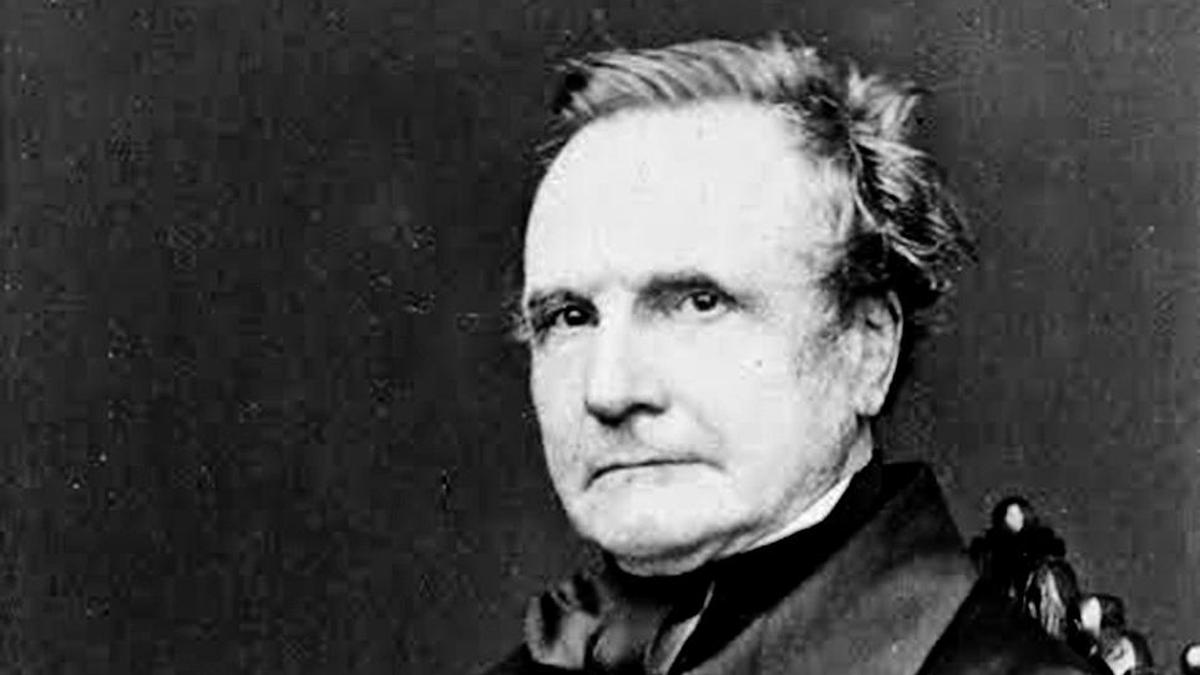
Modern computing is often effortless. You pick up a calculator or open the calculator app on your phone, and you’re on your way in seconds. But getting here took humans several centuries from when they first tried to speed up computing. One particularly important passage in this history involved the English mathematician Charles Babbage, who found a way to speed up calculations using the movement of simple machines, creating the first ancestors of the modern computer.What motivated Babbage?If you had to calculate something in the early 19th century, you had to do it entirely by hand. Entire governments, navigators, astronomers, engineers — all depended on complicated mathematical tables produced by teams of clerks, known at the time as ‘computers’, who worked slowly and often made mistakes.In 1821, Babbage was frustrated and reportedly said he wished calculations could happen “by steam”. Babbage went on to develop the difference engine, a large mechanical calculator designed to compute mathematical tables using a method called finite differences.The machine consisted of columns of brass wheels, each engraved with the digits from 0 to 9. The wheels physically added values as they were rotated using a hand crank and gears. The machine considerably reduced the number of mistakes. The difference engine was thus a specialised calculator that was fast and efficient at one class of problems.What were mathematical tables?The mathematical table was a pre-computed table of numbers that experts could refer to repeatedly in their practice. For instance, before digital calculators, an engineer would often convert multiplication into an addition problem using logarithms. So 247 x 83 could be solved by looking up the logarithms of both numbers, adding them, then converting back to the inverse value.Similarly, the tables also provided the values of trigonometric functions (used in architecture and civil engineering), astronomical tables (to predict the positions of celestial bodies), actuarial tables (for insurance and taxation), and polynomial tables (values of complicated functions used in science).The tables often repeatedly evaluated the values of common functions at regular intervals. For example, if f(x) = x3, then the tables would provide the values of f(x) at x = 1, 2, 3, 4, …, i.e. 1, 8, 27, 64, …. Similarly, a table would show the values of a trigonometric sine function for every tenth of a degree: 10°, 10.1°, 10.2°, … corresponding to 0.1736, 0.1754, 0.1771, ….Aside from computers making mistakes during the calculation itself, inaccuracies also crept up during copying and typesetting. And a single mistake could be ruinous.What is the method of finite differences?The method of finite differences simplifies many of these operations to simpler problems, which the difference engine could then automate.Say a table needs to evaluate the function f(x) = x2. So for x = 1, 2, 3, …, f(x) = 1, 4, 9, …. Now look at the differences between successive values: 3 (4 – 1), 5 (9 – 4), 7 (16 – 9), 9 (25 – 16), …. Then look at the second differences, i.e. the difference between the differences: 2 (5 – 3), 2 (7 – 5), 2 (9 – 7), ….That the second difference is a constant implies the whole table can be generated using just addition.The difference engine started with three numbers loaded into separate columns of wheels: the starting value, 1; the first first-difference, 3; and the second difference, 2. When you crank the wheels, they add the second difference to the first difference: 3 + 2 = 5 — and then the updated first difference to the current value: 1 + 5 = 6.At the end of turn 1:
How Babbage automated calculations with simple machines
Slow, error-prone calculations by hand were unavoidable in the early 19th century, yet even small mistakes could ruin the designs for buildings and the journeys of ships; Charles Babbage’s ingenious machines were much more accurate, faster, and revolutionary
1,540 words~7 min read