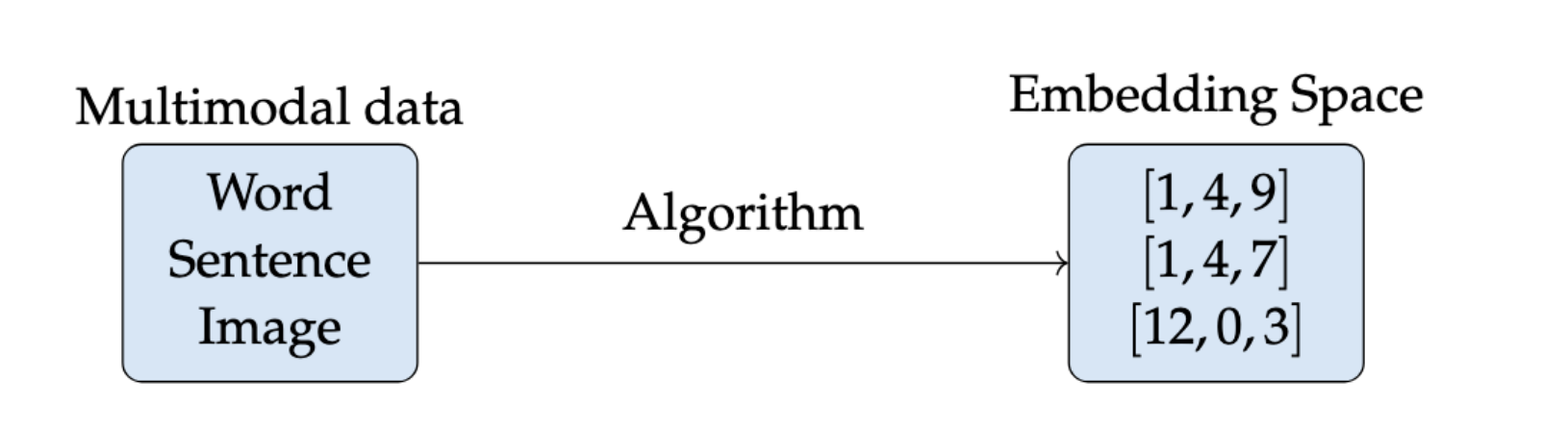
A few years ago, I wrote a paper on embeddings. At the time, I wrote that 200-300 dimension embeddings were fairly common in industry, and that adding more dimensions during training would create diminishing returns for the effectiveness of your downstream tasks (classification, recommendation, semantic search, topic modeling, etc.)I wrote the paper to be resilient to changes in the industry since it focuses on fundamentals and historical context rather than libraries or bleeding edge architectures, but this assumption about embedding size is now out of date and worth revisiting in the context of growing embedding dimensionality and embedding access patterns.As a quick review, embeddings are compressed numerical representations of a variety of features (text, images, audio) that we can use for machine learning tasks like search, recommendations, RAG, and classification. The size of the embedding is how many features our item has.For example, let’s say we have two butterflies. We can compare them among many dimensions, including wingspan, wing color, number of antennae. Let’s say we have a 3-dimensional feature for a butterfly, it might look like this.Doing a visual vibe scan, we can eyeball the data and see that butterfly_1 and butterfly_3 are more similar to each other than to butterfly_2 because their features are closer together.But butterflies are 3-dimensional animals and some of these features are numerical. When we talk about embeddings in industry these days, we generally mean trying to understand the properties of text, so how does this concept work with words? We can’t directly compare words like “bird” and “butterfly” or “fly” in a given text but we can compare their numerical representations if we map them into the same shared space. We can see that “bird” and “flying” are more similar to each other than to “dog” through their numerical representations.Intuitively, we know this is true, but how do we artificially create these relationships?There are different ways of creating text embeddings from a given word, all of which rely on analyzing that word in relation to the words around it in a given corpus of data. We can use traditional count-based approaches like TF-IDF based on term frequency in documents, or statistical approaches like PCA or LSA.With the advent of deep learning models, we started learning representations generated from models like Word2Vec that maximized the probability that a left-out word would be next to other given words in the training dataset.When we learn the embedding representation of a given word using probabilistic models, we are comparing how similar these words are to other words. Each feature is not an explicit feature like “wing color”, but rather a vibe-based latent representation in the latent space that doesn’t have a clear explanation.For example, one dimension might be “this word is an action word” or maybe “this word is related to other words about food”, but we generally don’t know exactly what the model thinks each feature represents. In fact, this is a fascinating area of study we are just starting to understand how these latent representations work through ideas like control vectors, a concept that Anthropic explored in the famous Golden Gate Claude paper.When we train a model, embedding size is initialized as a hyperparameter before model training, and we iterate on the size depending on our downstream evaluations after training. Picking the right hyperparameter is (alchemy) a combination of art and science and depends on optimizing training throughput, final embedding storage size, and the performance of the embedding on your downstream task both qualitatively and wrt to latency of performing search on embeddings of different sizes.Since previous generations of models were smaller and trained in-house, hyperparameters were usually not published by companies, and as such, there was no standard agreement on embedding size. We generally, as an industry, understood that somewhere around 300 dimensions for a given embedding model might be enough to compress all the nuance of a given textual dataset. 300 was the number of dimensions typically used by earlier models like Word2Vec and GloVE.After the publication of the attention paper BERT was released in 2018. This model’s architecture introduced embeddings of 768 dimensions. Although previous RNN and LSTM models had been trained on GPUs, BERT was one of the first larger embedding models to be trained on GPUs (and TPUs), which meant that GPU optimization now became increasingly important.The key behind training Transformer models efficiently is the ability to efficiently move data onto GPU and parallelize their matrix multiplication operations between several pipelines, aka attention heads, where each attention head can focus on understanding and defining a different part of the embedding feature space. As such, the embedding needs to be able to be partitioned evenly between the number of attention heads.BERT has 12 attention heads, so 768 dimensions was selected from a combination of trial and error and efficiently parallelizing computation to “attend” to different parts of the feature space, meaning that, in model training, each head operates on a 64-dimensional subspace of the original 768-dimensional input embedding. This itself comes from the Transformer paper, where each sub-embedding size per head is commonly chosen as 64.As a result, many BERT-style models, and related model families, used 768 as a baseline for embedding dimensions. Although it had a much larger training dataset, GPT-2 also implemented 768. And, although CLIP uses an embedding size of 768 as derived from the Vision Transformer architecture that CLIP uses for its image encoder, and for consistency, the text encoder also uses this dimension size[^1].Even though training cycles for BERT were fairly small (4 days for the original BERT model) compared to the months-long pretraining processes that LLMs require these days, it was still hard computationally to infer these embedding sizes, even with GPU optimizations. For BERT, for example,Finding the most similar pair in a collection of 10,000 sentences requires about 50 million inference computations (~65 hours).
How big are our embeddings now and why?
Embedding sizes and architectures have changed remarkably over the past 5 years
1,667 words~8 min read