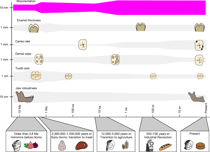
MainEnamel-like tooth structure is common to nearly all vertebrates and has been evolving since it first appeared in conodonts nearly 400 million years before present (bp)11. Enamel varies and evolves at multiple structural levels and developmental stages.The structure and properties of enamel differ at different scales. At the macroscale, the thickness and shape of enamel can evolve quickly in response to the mechanical properties of food12,13. For example, teeth that have thick enamel14 and blunt cusps are adapted to hard and abrasive foods, whereas teeth with thin enamel wear obliquely and have shearing edges suited for slicing soft foods13,15.Hard-food consumption is associated with several dental adaptations in modern primates that resist crack propagation, including large teeth, low-crowned molars and premolars, and thick, unevenly distributed enamel13,16,17. Thick enamel at the millimetre scale helps prevent crack nucleation18.At the micro- and nanoscales, enamel structure evolved to limit crack widening and propagation, thereby improving fracture resistance, also known as fracture toughness, or simply toughness3,19. At the microscale, decussating enamel prevents cracks from widening and propagating by deflecting them20 at the interface between rod and interrod enamel21. At the nanoscale, researchers originally incorrectly assumed that adjacent nanocrystals within rods are co-oriented because they elongate parallel to one another morphologically, but they actually vary in orientation22. The angular distance of crystallographic c-axes in adjacent nanocrystals can vary by tens of degrees, and their orientation gradually changes within and across each rod by as much as 30–90° (ref. 22). Hereafter, we term this non-zero angular distance between the c-axes of adjacent nanocrystals simply ‘misorientation’. Molecular dynamics simulations have shown that misorientation deflects cracks and therefore toughens tooth enamel22.The enamel formation mechanism, comprising organic matrix deposition, amyloid-like nanoribbons23, subsequent mineralization and resorption of the organic matrix, is conserved across all mammals, including primates24. Although primates differ in size (teeth, mouths, bodies, brains) and developmental rates25, they do not differ in enamel rod size, the presence of decussation patterns or nanocrystal sizes26. Thus, it is possible to make controlled comparisons of adjacent enamel nanocrystals across species without confounding size and developmental factors.Dietary shifts coincide with dental changesWe investigated whether crystalline nanostructure and orientation changed with dietary hardness across primates, with particular emphasis on hominins, that is, members of the human lineage, including modern humans and our extinct fossil relatives. Supplementary Table 1 provides a summary of the terms frequently used for primates, including hominins, and to which group each of the nine species analysed in this study belongs. Supplementary Table 2 documents the 12 samples in this study.After diverging about 4–8 million years bp from the last common ancestor with chimpanzees27,28, hominins began incorporating meat into their diet about 2.0–1.5 million years ago (Ma); humans invented agriculture around 12,000 years bp, adopted it widely in the later Holocene, and ramped up production of processed food during the Industrial Revolution beginning around 250 years bp. During the past 2 million years of human evolution, teeth became smaller29 with thinner enamel layers30 and more pronounced decussation31,32. These dental changes occurred alongside brain expansion33, increased body size34, reduced facial and oral structures35, language development36, and cultural expansion37. Figure 1 documents significant changes in the size of human teeth, enamel thickness, wear patterns and caries prevalence following each major shift in human diet and technological advance (see Supplementary Tables 3–8 for references).Fig. 1: Hominin dentitions have changed in relation to dietary changes over the past 10 million years.The alternative text for this image may have been generated using AI.Full size imageSince hominins diverged from the last common ancestor shared with chimpanzees, significant dental changes occurred over the millimetre-to-centimetre scales. Compared with the earliest hominins, modern humans have less robust jaws, smaller posterior teeth and thinner enamel, as well as less occlusal wear but greater caries prevalence (10 cm−1 mm, previous work; all references and details are presented in Supplementary Tables 3–8). At the nanoscale (10 nm), modern humans have more misoriented enamel than the earliest hominins, as reported here in magenta (this work).Nanocrystal misorientation in PELICANTo determine whether the millimetre-to-centimetre-scale structural changes summarized in Fig. 1 were accompanied by nanoscale changes in c-axis crystal misorientation, we examined 12 polished histological cross-sections of primate molar or premolar teeth from fossil, archaeological and modern ape and monkey species (Supplementary Table 2). We analysed variations within a species and across species, and tested correlations with dietary hardness and time. The 12 samples included two Miocene primates (Ekembo heseloni and Victoriapithecus macinnesi, 17.8 Ma and 14 Ma), three Early Pleistocene hominins (Paranthropus boisei, Homo habilis and Homo erectus), four Homo sapiens spanning pre-agricultural to modern times (pre-agriculture about 40,000 years bp, two agricultural British archaeological samples from 1,550 years bp and 700 years bp, and one modern human), and three extant primates with markedly different diets (Pan troglodytes, Pongo pygmaeus and Cercocebus atys). The H. sapiens samples track temporal trends across 40,000 years, including dietary differences (pre-agriculture versus agriculture), and variation within groups (two pre-modern, agricultural samples and one modern sample). We used a method called Polarization Enabled Large Input of Crystal Angles at the Nanoscale (PELICAN), developed for this work, on sets of photoemission electron microscopy (PEEM)38,39 images. These ‘datasets’ were acquired similarly to polarization-dependent imaging contrast mapping40, but with revised image normalization and data processing that increases precision and provides high-throughput c-axis orientation information for every pixel. See Supplementary Methods for details. Extended Data Fig. 1 compares a PELICAN map with other imaging methods showing precisely the same region of enamel.Using PELICAN, we compared the misorientation angle in three-dimensional space of two adjacent 50-nm pixels, matching the smallest possible size of enamel nanocrystal, which is also 50 nm. We compared each pixel with its adjacent eight pixels, identified the maximum misorientation angle and recorded that angle value. Choosing the maximum misorientation excludes co-oriented adjacent pixels and nanocrystals. We then produced a histogram of 1 million maximum misorientation angles per dataset, and 9 partly overlapping datasets for each area analysed (Extended Data Fig. 2). We calculated the mode, width and footprint of each misorientation histogram to enable statistical comparison. Each PELICAN histogram therefore represents 9 million maximum misorientations, derived from 72 million pixel-pair comparisons per area. We repeated this analysis on the occlusal side of each tooth (Extended Data Fig. 2), and produced 3 × 3 partly overlapping PELICAN maps, in which colour quantitatively represents the orientation of the crystallographic c-axis in each pixel.The full set of data and histograms is provided in the Supplementary Data 1. We used non-parametric tests to assess the significance of each comparison, owing to small sample sizes and a few non-normal distributions (Supplementary Table 9). Therefore, we used Kruskal–Wallis tests for pairwise comparisons between groups and Jonckheere–Terpstra tests to evaluate hypotheses of ordered, directional trends across dietary hardness categories and time; all P values were Bonferroni-corrected where multiple comparisons were made. In Fig. 2, we present a summary of occlusal area results from all samples, along with representative skulls and reconstructions of faces for all species, drawn to scale with respect to one another, the size and shape of a molar tooth for each species, the foods each primate ate or eats, and the average and standard deviation across nine datasets of the most frequently occurring (mode) misorientations measured. Supplementary Tables 5–8 document what is known about the mechanical properties of each species’ diet.Fig. 2: Samples represent primates across time, taxa and diet.The alternative text for this image may have been generated using AI.Full size imagea, Archaeological and fossil samples are presented by epoch (black horizontal lines represent epoch borders; red horizontal lines represent sample ages): E. heseloni (Eh) and V. macinnesi (Vm) date to the Miocene, P. boisei (Pb), H. erectus (He), H. habilis (Hh) and the pre-agricultural H. sapiens (PA) date to the Pleistocene, and two agricultural H. sapiens (Arch1 and Arch2) date to the Holocene (Supplementary Table 2). b, All locations of origin are indicated on the world map alongside a representative lower molar, skull and partial reconstruction. The grey scale bar for skulls is 50 mm; the beige scale bar for molars is 5 mm (Supplementary Table 2). c, The misorientation mode averaged over nine acquisitions in each sample; error bars are 1 s.d. (Supplementary Data 1). Extant species are abbreviated P. troglodytes (Pt), P. pygmaeus (Pp), modern human H. sapiens (MH) and C. atys (Ca). Arch1 and Arch2 are abbreviated A1 and A2. Credit: world map by Clker-Free-Vector-Images via Pixabay.Misorientation increases with diet hardnessFirst, we sought to establish whether and how enamel nanocrystal misorientation varies with dietary hardness. To do this, we compared misorientation histograms from species with a range of dietary hardnesses: P. troglodytes, P. pygmaeus, P. boisei, V. macinnesi, E. heseloni and C. atys. Figure 3g reveals that (1) C. atys, a dedicated hard-object feeder, is significantly different from all the other species (Supplementary Table 10); (2) V. macinnesi and E. heseloni show nearly identical histograms despite one being a monkey and another an ape; (3) P. pygmaeus and P. boisei plot together and are both known to consume a diet including tough objects; (4) P. troglodytes has significantly lower misorientation.Fig. 3: Cercocebus atys misorientation is significantly greater than that of all other fossil and modern apes and monkey.The alternative text for this image may have been generated using AI.Full size imagea–f, PELICAN maps of two modern apes, P. troglodytes (Pt) (a) and P. pygmaeus (Pp) (b); and one modern monkey, C. atys (Ca) (c); two fossil apes, E. heseloni (Eh) (d) and P. boisei (Pb) (e); and one fossil monkey, V. macinnesi (Vm) (f). Sample abbreviations are in the Fig. 2 caption. Scale bars, 5 μm. θsp and φsp are the spherical polar coordinates of the crystalline c-axis. They display in colour and grayscale, respectively, the in-plane and out-of-plane orientation angles of the c-axis vector. g, Normalized histograms of misorientation for each of the samples in a–f. h, The histogram parameters averaged over nine datasets per area. Statistics: Kruskal–Wallis two-tailed Bonferroni significance is calculated based on 15 comparisons of 6 samples, each with nine datasets per area; *P < 3.3 × 10⁻³ (0.05/15), **P < 6.7 × 10⁻⁴ (0.01/15), ***P < 6.7 × 10⁻⁵ (0.001/15). All Kruskal–Wallis P values are in Supplementary Table 10.Both V. macinnesi and E. heseloni likely consumed primarily fruit and have statistically indistinguishable misorientation histograms with modes of 2.5° and 2.7°, respectively41,42 (Kruskal–Wallis, P = 0.591; Fig. 3). P. boisei falls between the modern (P. troglodytes and P. pygmaeus) and fossil (E. heseloni) apes and only differs significantly from C. atys. The misorientation mode, width and footprint of C. atys are significantly greater than those of all other samples (Kruskal–Wallis, all P < 8.3 × 10⁻³; Supplementary Table 10).P. troglodytes and C. atys show the lowest and highest misorientation angles, respectively, at 1.3° ± 0.4° and 7.2° ± 1.7°, which represents a 6-fold difference (Kruskal–Wallis, P = 7.5 × 10⁻¹¹; Figs. 2c, 3 and Supplementary Table 10). These two species have the most distinct diets: P. troglodytes occasionally eats meat or termites, but mostly consumes ripe fruit43, whereas C. atys feeds preferentially on the oily seeds of Sacoglottis gabonensis trees, which it cracks with its enlarged molars and premolars. The nutshell-like-casing of the seeds is very hard and stiff, requiring powerful isometric bites to crack44,45. The high misorientation mode and heterogeneity in C. atys, combined with its specialized hard-object diet, suggest that greater misorientation is an adaptation to more mechanically challenging diets. This nanoscale pattern mirrors known macroscale adaptations: C. atys evolved thicker enamel and larger molars for hard-food processing, whereas P. troglodytes evolved molars with thinner enamel to maintain sharp cutting edges15. These data suggested a trend of misorientation with food hardness that needed further validation.From each set of 9 million misorientations per sample in Fig. 3, we compared mode, width and footprint of the histogram and found that they all increased with hardness of food. All three histogram parameters increased significantly with dietary hardness across both the full non-hominin comparison (6 samples, 54 histograms) and an extant-only subset (3 samples, 27 histograms; Jonckheere–Terpstra, all P < 5 × 10⁻⁴; Fig. 4a–c and Supplementary Table 11). This positive directional trend indicates that misorientation (mode) increases and becomes more heterogeneous (width, footprint) as dietary hardness increases from softest to hardest (Fig. 4a–c). Significant pairwise differences were observed between the softest diets and those of V. macinnesi and E. heseloni categories, between soft and very hard diets, and between intermediate and very hard diet categories (Kruskal–Wallis; Supplementary Table 10).Fig. 4: Enamel nanocrystals are more misoriented and heterogeneous when diets include harder foods.The alternative text for this image may have been generated using AI.Full size imagea–c, Misorientation histogram parameters, mode (a), width (b) and footprint (c), for the six non-hominin primate samples from Fig. 3, ordered by increasing dietary hardness (Fig. 3): P. troglodytes (Pt, soft, dark blue), P. pygmaeus (Pp, tough, yellow), P. boisei (Pb, tough, yellow), V. macinnesi (Vm, unknown hardness, magenta), E. heseloni (Eh, unknown hardness, magenta), C. atys (Ca, very hard, cyan). d, Boxplot of PC1 factor scores plotted versus dietary hardness categories: soft (dark blue, Pt), intermediate (yellow, Pp, Pb), Vm, Eh (magenta, unknown fossil taxa with unknown diets), and very hard (cyan, Ca). Statistics: box plots show median, interquartile range and range. Kruskal–Wallis comparisons identify significant differences between dietary groups, denoted by black bars and asterisks. Kruskal–Wallis two-tailed Bonferroni significance was calculated based on six comparisons of four dietary hardness categories; *P < 8.3 × 10⁻³ (0.05/6), **P < 1.7 × 10⁻³ (0.01/6), ***P < 1.7 × 10⁻⁴ (0.001/6). All Kruskal–Wallis P values can be found in Supplementary Table 12.As mode, width and footprint are independent histogram parameters, but they all similarly increase with hardness (Fig. 4a–c), we used principal component analysis (PCA) to obtain a single principal component (PC1) capturing the magnitude (mode) and heterogeneity (width and footprint) in misorientation with one component or dimension. Mean PC1 factor scores ranged from −0.95 (median −1.02) for soft diets to +1.94 (median 2.18) for very hard diets, effectively separating food hardness categories (Fig. 4d, and Supplementary Tables 11 and 12). PC1 factor scores increased significantly as dietary hardness increased in extant samples (Jonckheere–Terpstra, P = 1.8 × 10⁻⁷; Supplementary Tables 11 and 12), consistent with the pairwise comparisons of harder and softer diets in Fig. 3h and Supplementary Table 10.Genus Homo misorientation and dietHaving established the misorientation versus hard-food trend, we analysed 7 hominins, fossil and modern, that span approximately 1.6 million years and 3 major dietary shifts. Misorientation mode differed significantly between P. boisei and both H. erectus and H. habilis (Kruskal–Wallis, P = 1.5 × 10⁻² and P = 1.7 × 10⁻³, respectively; Fig. 5). Despite living at the same time (1.6–1.8 Ma) and in the same place (Koobi Fora, Kenya), P. boisei had lower misorientation mode than either early Homo samples, whereas H. erectus and H. habilis misorientations were statistically similar to one another in mode, width and footprint (Kruskal–Wallis, P > 0.05; Fig. 5). Thus, we can identify a correlation between meat-eating and misorientation, with modes increasing from 2.1° ± 0.1° (Pb) to 3.1° ± 0.2° (H. erectus) (Figs. 2 and 5). H. habilis ate meat but not as regularly as H. erectus, yet this hominin had slightly more misoriented nanocrystals, with a misorientation mode of 3.5° ± 0.3° (Kruskal–Wallis, P = 0.488). We found no discernible difference between the fossil ape and monkey (E. heseloni and V. macinnesi), but differences in misorientation were observable in the later hominins (P. boisei,H. habilis and H. erectus; Kruskal–Wallis; Fig. 5f). Taking into consideration the significant relationship between misorientation and hard foods identified in primates (Figs. 3 and 4), the increase in misorientation with the introduction of meat (Fig. 5) can be interpreted as meat-eating being more challenging for enamel, because meat is tougher than fruit.Fig. 5: The consumption of meat in hominin diets correlates with an increase in misorientation angle.The alternative text for this image may have been generated using AI.Full size imagea–c, PELICAN maps of the occlusal enamel region from P. boisei (Pb; no meat; a), H.erectus (He; regular meat consumption; b) and H. habilis (Hh; occasional meat consumption; c). Scale bars, 5 μm. d, Normalized histograms of misorientation for each area. e, Histogram parameter averages for each sample. f, Kruskal–Wallis (KW) test P values comparing the histogram parameters from nine datasets per area across species. Kruskal–Wallis two-tailed Bonferroni significance is calculated based on three comparisons of three samples; *P < 1.7 × 10⁻² (0.05/3), **P < 3.3 × 10⁻³ (0.01/3), ***P < 3.3 × 10⁻⁴ (0.001/3).Figure 6 documents misorientation changes in H. sapiens from a pre-agricultural individual from Spain (PA, around 40,000 years bp), two British archaeological samples from agricultural populations (Arch1, around 1,550 years bp, and Arch2, around 700 years bp), and a recent clinically extracted molar from a modern British individual (around 50 years bp). Unexpectedly, the pre-agricultural misorientation mode, width and footprint are significantly lower than those of any more recent agricultural or industrial H. sapiens. Thus, the transition to grain-based agriculture in Europe around 12,000 years bp correlated with a significant increase in enamel nanocrystal misorientation. Misorientation mode was significantly higher in Arch1 than the pre-agricultural individual (4.7° ± 0.1° versus 2.5° ± 0.1°; Kruskal–Wallis, P = 2.9 × 10⁻³; Supplementary Table 13). Comparison of the pre-agricultural individual with Arch2 yielded very similar results, with misorientation mode at 4.6° ± 0.5° (Kruskal–Wallis, P = 3.9 × 10⁻³; Supplementary Table 13). The misorientation of crystals in the 2 archaeological teeth is almost double (1.9- or 1.8-fold) that of the pre-agriculture tooth. Following the transition to agriculture, Arch1, Arch2 and modern human H. sapiens (MH) showed consistent misorientation modes around 4.7°, with no significant pairwise differences among them (Kruskal–Wallis, all P > 0.05; Fig. 6 and Supplementary Table 13). The more recent Industrial Revolution did not result in a significant change in misorientation, although increases in caries and dental crowding indicate other dental consequences of an industrialized diet over the past 250 years10,46. This demonstrates that this 4.6–4.8° misorientation mode has remained stable for the past 1,550 years, at least in agricultural Britain.Fig. 6: Transition to agriculture correlates with increased misorientation, whereas the Industrial Revolution produced no significant change in misorientation.The alternative text for this image may have been generated using AI.Full size imagea–d, PELICAN maps of H. sapiens: PA (pre-agriculture; a), Arch1 (b) and Arch2 (c) (post-agriculture, pre-Industrial Revolution), and MH (post-Industrial Revolution; d). Sample labels and abbreviations are at the top of all PELICAN maps. Scale bars, 5 μm. e, Normalized histogram for each area in a–d. f, Kruskal–Wallis tests reveal significant differences between the histogram parameters of different samples, again from nine datasets per sample. Kruskal–Wallis two-tailed Bonferroni significance is calculated based on 6 comparisons of 4 samples; *P < 8.3 × 10⁻³ (0.05/6), **P < 1.6 × 10⁻³ (0.01/5), ***P < 1.7 × 10⁻⁴ (0.001/6). All sample comparison (PA, Arch1, Arch2, MH) Kruskal–Wallis P values can be found in Supplementary Table 13. g, The PC1 factor scores for samples grouped into four time periods: early Homo (light blue, H. habilis and H. erectus), pre-agriculture (pink, PA), agriculture (purple, Arch1 and Arch2) and today (dark grey, MH). The box plot shows median, interquartile range and range. Outliers (falling within 3 times the height of the interquartile range) are noted by circles and extreme values (falling further than 3 times the height of the interquartile range) are stars. Kruskal–Wallis comparisons identify significant differences between time periods (denoted by black bars and asterisks; Bonferroni-corrected thresholds for 6 comparisons; *P < 8.3 × 10⁻³ (0.05/6), **P < 1.6 × 10⁻³ (0.01/6), ***P < 1.7 × 10⁻⁴ (0.001/6); full P values in Supplementary Table 16).Over the past 1.76 million years of Homo evolution, though, we can identify a trend towards increasing misorientation angles (Supplementary Table 14 and Extended Data Fig. 3). This trend stands out clearly when Homo misorientation is compared over time (Fig. 6g). PC1 factor scores increased significantly across four major time categories: early Homo, pre-agricultural H. sapiens, archaeological H. sapiens and modern humans (Jonckheere–Terpstra, P = 5.0 × 10⁻⁵; Supplementary Tables 11 and 14). Although the composite PC1 misorientation factor score decreased between around 1.7 million years bp (Hh and He) and 40,000 years bp (PA) (Fig. 6c, Supplementary Fig. 16 and Supplementary Table 16), the trend is still very significant (Supplementary Table 14 and Extended Data Fig. 3). Pairwise comparisons of the individual parameters reveal similar results, with misorientation mode, width and footprint all differing significantly when pre-agriculture is compared with agriculture and today (Kruskal–Wallis, P < 1.7 × 10⁻⁴; Supplementary Table 13). Between early Homo and agricultural and today, only mode differed significantly (Kruskal–Wallis, P < 1.6 × 10⁻³; Supplementary Table 13), and between early Homo and pre-agriculture, only footprint differed (Kruskal–Wallis, P = 6.9 × 10⁻⁴; Supplementary Table 13). The tight correlation among misorientation mode, width and footprint (Supplementary Table 15) suggests that as misorientation increases (mode), so does the misorientation heterogeneity (width and footprint). Many other parameters were tested and found to not correlate with mode, width and footprint misorientations, nor with one another (Supplementary Table 15). The PC1 comparison, therefore, allows quantitative evaluation of misorientation change over time within the genus Homo (Extended Data Fig. 3 and Supplementary Tables 14–16).Misorientation within and across teethThe results found in recent humans with an agricultural diet (≤1,550 years bp) indicate that misorientation is consistent across individuals within a group. We obtained the Arch1 and Arch2 results from the functional cusp of a lower and upper first molar, respectively, suggesting that teeth on the upper and lower jaw have consistent misorientations. Within a tooth, the rod and interrod enamel crystals are oriented differently from one another; therefore, they differ in colour in PELICAN maps. However, when the misorientation of adjacent nanocrystals within rods and interrod enamel in the same area is compared, they are not statistically distinct (Kruskal–Wallis, all P > 0.05; Extended Data Fig. 4). We established this using the two samples with the most extreme diets: the most misoriented C. atys and the least misoriented P. troglodytes. Separating rods from interrod enamel across species, therefore, does not change any of the above results. Supplementary Data 2 provides all the data relevant to this comparison.For three samples (PA, MH and Eh), we acquired and compared two PELICAN areas, on the occlusal and lateral sides of the dentin horn (Extended Data Figs. 2, 5 and 6). We found no significant differences in misorientation histogram parameters for the pre-agricultural and most recent human (Kruskal–Wallis, all P > 0.05; Extended Data Fig. 5) and E. heseloni (Kruskal–Wallis, all P > 0.05; Extended Data Fig. 6) between occlusal and lateral sides. Therefore, the misorientations in decussating enamel on occlusal and lateral sides of a dentine horn of a functional cusp of one tooth are probably representative of decussating enamel under all functional cusps of all molar and premolar teeth. The four H. sapiens teeth demonstrate that misorientations are also probably representative of all teeth in the same species. Therefore, the comparison of misorientation in occlusal areas done across all 12 samples in this study is well supported.For the oldest sample, E. heseloni, we also analysed a region of radial enamel near the cusp tip and found that misorientation mode, width and footprint were greater in radial than in decussated enamel (Kruskal–Wallis, all P < 0.017; Extended Data Fig. 6). This contrasts with previous observations showing that enamel at the outer enamel surface (aprismatic and radial) exhibited lower toughness than the decussated enamel near the dentin-enamel junction47. However, none of the comparisons in this work are based on radial enamel, only on decussating enamel.Closing thoughtsThe primary observation described here is that the misorientation of adjacent nanocrystals changed in conjunction with dietary shifts and, within the human lineage, misorientation increased when hominins introduced both meat and agricultural products into their diet. This observation suggests that nanocrystal misorientation may contribute to a tooth’s resilience against hard or tough foods, complementing previously documented adaptations such as tooth size, shape, enamel thickness and microstructure that confer resistance to wear and/or crack propagation. Thus, dietary specialization drives evolutionary changes across multiple hierarchical levels of enamel structure, down to the nanoscale.The nut-cracking C. atys has an extremely mechanically demanding diet that requires the most resilient teeth44,45. We found that this monkey also has the greatest misorientation and exhibits the widest range of misorientation of all teeth measured (Figs. 3 and 4). We tentatively conclude, therefore, that we can add nanoscale misorientation to the suite of macro- and microscale adaptations that make enamel either harder, stiffer or tougher, or a combination of these material properties in relation to more mechanically challenging diets.Although foods became easier to masticate over human evolutionary history with improvements in food processing and cooking48,49, we find that misorientation increased across both the transitions to meat-eating and agriculture. To test whether the misorientation shifts observed in Homo reflect factors other than diet, we calculated correlations between misorientation and sample age, tooth size, enamel thickness, maximum bite force and surface microwear values, but identified no significant correlations (Spearman’s rho, all P > 0.05; Supplementary Table 15). Ruling out those other factors, we returned to diet. One possible cause for the observations here might be that greater misorientation compensated for the marked and continuing reduction in molar size that characterizes our human lineage (Fig. 1). And, although agricultural food products may be more processed, the by-products of that processing (for example, millstone grit) may have contributed to high abrasion and significant wear in recent modern humans17.We note that, even if greater misorientation is better from a materials perspective, all angles measured in all 12 samples were small misorientation angles, with modes between 1° and 7°, widths between 2° and 9°, and even the footprints of all histograms were small angles, between 4° and 18°. These misorientation angles fall within what material scientists call low-angle boundaries, which are typically defined as <15°. Such low-angle grain boundaries are low-energy surfaces, with surface energy of approximately 1 J m−2, increasing monotonically with misorientation angle50. This excess energy hinders dislocation motion, and thus stabilizes nanostructures50. Low-angle boundaries could have a similar role in ionic crystals such as hydroxyapatite or calcium carbonates, for example, under grinding conditions common for posterior teeth. Intriguingly, in molybdenum disulfide51 and graphene52, low-angle grain boundaries have materials properties strongly dependent on misorientation angle. The results presented here, particularly the contrast between the fruit-eating chimp and the nut-cracking monkey, suggest a strong dependence of mechanical properties on misorientation angle.MethodsSampleThe nine species analysed in this study are listed in Supplementary Table 1. The 12 tooth samples, locations of origin, date, collection ID and precise tooth analysed are listed in Supplementary Table 2. Whenever possible, we selected lower first molars (LM1) and the mesio-buccal cusp, which experiences crushing and grinding forces and is the first to wear53,54 (Extended Data Fig. 2). When an LM1 was not available (for example, fossil samples), we used the functional cusp of the available molar or premolar, which is equivalent to an LM1’s mesio-buccal cusp in its masticatory function (Extended Data Fig. 2). In all cases, analysis was restricted to molar or premolar teeth and focused on the occlusal region proximal to the dentine horn to control for functional use and avoid worn enamel.Histological sample preparationPrevious studies generated histological sections of PA, Arch1, Arch2, MH, Pt, Pp and Ca, but all used a standard set of histological methods55,56. Details of materials and consumables used for each sample can be found in their respective published articles (Supplementary Table 2). We identified no pathologies or taphonomic features in any sample. When wear was present, it was minimal and did not reach the dentine horn. All samples are permanent posterior teeth from adult individuals, with the exception of Ca, which was a subadult. Teeth were embedded in epoxy resin before being sectioned. Each tooth was sectioned through a plane intersecting the two mesial cusps (in the case of premolars, the two primary cusps; Extended Data Fig. 2) using a precision saw. The section was mounted on a microscope slide and used for other studies. For this study, we used the ‘off-cut’, which is the remaining portion of the tooth that was not mounted to the microscope slide. This off-cut was re-embedded, ground and polished as described below (‘Sample preparation for PEEM’).The histological sectioning and analysis of the Eh sample was published in ref. 57; Vm was published in ref. 58; Hh, He and Pb were published in ref. 59. C. M. Dean led the histological preparation for these five samples, following standard protocols55,56. For these samples, no pathologies or taphonomic features were identified; when wear was present, it was minimal and did not reach the dentine horns.Sample preparation for PEEMSamples arrived sectioned; we re-embedded, then ground and polished them. For re-embedding, we soaked blocks or slides in anhydrous ethanol and placed them face-down in two-part plastic moulds (Ted Pella) and covered them with freshly mixed EpoFix (EMS; 25 g epoxy, 3 g hardener, mixed with a Thinky planetary mixer, mixing for 1 min and defoaming for 1 min. We cycled the moulds three times through vacuum with a diaphragm pump kit (Ted Pella) and vented with nitrogen, to remove ethanol, ensure full epoxy penetration and burst surface bubbles. EpoFix cured overnight in air.All grinding and polishing used water as a coolant, but supersaturated with either 1 g l−1 CaCl2 or 0.2 g l−1 Na3PO4 (pH 9) in MilliQ water to prevent hydroxyapatite dissolution, dispensed by a peristaltic pump (Drive MFLX07522-30, Head MLFX07519-06, Tubing MFLX96410-14, all by MasterFlex, Avantor). We ground tooth surfaces with 600, 1,200 and 4,000 grit SiC paper (Buehler) using 5 N, 30 s each, 40/140 rpm co-rotating on a Buehler AutoMet 250 PM. We then polished the tooth surfaces on the same Buehler AutoMet 250 PM with 300-nm alumina (MicroPolish 0.3 µm, Buehler) using 10 N, 2 min, 40/140 rpm counter-rotating, then with 50-nm alumina (MasterPrep, Buehler) with 10 N, 1 min, 30/30 rpm counter-rotating. Both 300-nm and 50-nm suspensions were dispensed automatically via burst modules (Buehler). This protocol yields mirror-flat surfaces with ≤1 nm residual roughness, as previously verified by atomic force microscopy. When possible, we thinned the samples to 2 mm thickness, which is ideal for PEEM experiments. For the fossil samples (Vm, Eh, Hh, He and Pb) this was not possible; thus, we used a modified sample holder for the PEEM experiment. We trimmed the epoxy blocks to remove excess EpoFix resin and then cleaned them repeatedly with anhydrous ethanol and a new TexWipe Dry Cotton Cleanroom Wiper using gentle force until clean under differential interference contrast (DIC) microscopy (×20 objective). This step is key to obtaining perfect surfaces for the surface-sensitive PEEM method.We then transferred all samples to ultrahigh vacuum (approximately 10−8 mbar) to remove any residual water. Several samples took many hours to outgas: we attempted the PA sample during 3 beamtimes over 2 years and it failed until we built a dedicated ultrahigh-vacuum chamber, called the Dalì chamber (Supplementary Fig. 1). The ultrahigh-vacuum chamber included a 660 l s−1 turbo pump ceramic-bearing turbomolecular Agilent Twistorr 704 (Agilent Technologies). The pump is mounted at the bottom of the Dalì chamber, equipped with a fast-entry flange on a side, and a drawer that comes out to receive the sample, and goes back into the chamber directly above the turbo, where the sample sits while pumping down.We coated all samples twice using a Cressington 208HR (Cressington, Ted Pella) sputter coater. First, we coated the samples with 40 nm platinum and a 4 mm × 4 mm silicon wafer mask (MTI) to cover the functional cusp of the tooth and expose everything else to platinum, with no motion of the sample stage. Then, we removed the silicon mask and coated the whole sample with 1 nm platinum while spinning and tilting it. This coating method makes it possible to analyse with photoemission spectroscopy and microscopy any insulating sample including minerals60, biominerals61,62 and most importantly enamel22,63,64,65,66. At the calcium L edge, the maximum probing depth of the PEEM experiment is 3 nm (ref. 67); hence, a 1-nm coating enables much of the signal to originate from the sample under investigation. The 40 nm surrounding coating ensures good electrical contact between sample and sample holder, so that the sample can float at −18 kV without arcs and sparks, and the photoelectrons it emits can be accelerated towards the electrostatic optics column.We defined the region of interest identically in all samples. Whenever possible, we focused PELICAN analysis on specific occlusal regions of lower first molars (LM1) near the dentine horn to control for functional use, and selected the mesio-buccal cusp of each tooth because this region experiences both crushing and grinding forces53,54 (Extended Data Fig. 2). When an LM1 was not available (for example, fossil samples), we used the ‘functional cusp’ of the available molar or premolar, which is closest in its masticatory function to an LM1’s mesio-buccal cusp (Extended Data Fig. 2). The region selected for analysis in all tooth cross-sections was well below the surface of the functional cusp tip; the region of interest was approximately 200–300 µm occlusal to the apex of the dentine horn where both parazones and diazones of Hunter–Schreger bands in the decussation pattern were visible (Extended Data Fig. 2). We also analysed regions 200–300 µm lateral to the apex of the dentine horn for some samples. We precisely recorded the precise location of each area analysed in PEEM into a high-resolution optical image of each sample using Adobe Photoshop. Extended Data Figs. 5c and 6c, and Supplementary Fig. 2c provide examples of this precise localization in Photoshop, including the tooth cusp, the dentine horn, and the location of occlusal and lateral areas analysed with PEEM. The optical images were obtained with either DIC microscopy68 or polarized light microscopy (PLM), and show the whole sample surface. Extended Data Figs. 5c and 6c, and Supplementary Fig. 2c show examples of the DIC images. The PLM images used crossed polarizers on the illumination and reflected light channels at 90° ± 30° from one another. All DIC and PLM images were acquired using a Zeiss Axioscope 7 (CTK Instruments) and stitched together automatically using the Zeiss software.Scanning electron microscopyWe acquired scanning electron microscopy (SEM) images using a Zeiss EVO LS10 microscope, operated at 10 kV accelerating voltage and 9.5 mm working distance, in either secondary electrons or backscattered electrons mode. The SEM images in Extended Data Fig. 1 present both the secondary electrons or the backscattered electrons of the same region of a Ca sample. We imaged the sample as it had been coated for the PEEM experiment; thus, the SEM, PEEM and PELICAN images are all directly comparable from precisely the same sample and accurately the same region of sample surface, even though the greater penetration and scattering depths in SEM and the larger depth of field provide the impression of more topography in SEM than in surface-sensitive PEEM.PEEM beamtime experimentsWe acquired all data using the PEEM-3 microscope at the Advanced Light Source at Lawrence Berkeley National Laboratory. PEEM-3 is the end-station of beamline 11.0.1.1 at the Advanced Light Source and is a photoemission electron microscope38,39, with the sample floating at high voltage (−18 kV), fully electrostatic lenses69 magnifying the image formed by photoemitted electrons under soft-X-ray illumination, and a best resolution of 20 nm (ref. 40).PEEM-3 has an elliptically polarizing undulator source, which enables rotating the linear polarization of the soft-X-rays illuminating the sample surface. For this work, we acquired stacks of 38 full-field PEEM images while rotating the polarization from horizontal to vertical in 5° intervals. At each of 19 polarizations, we acquired 2 images at 2 photon energies on either side of the sharpest and most intense calcium L2 peak, termed peak 1, typically at 352.6 eV. We acquired the 2 images either 0.2 eV above and below peak 1, or +0.1 and −0.3 eV, whichever gave the greatest contrast in ratio images at each particular beamtime22,65. Both settings are effective, but the optimal choice varies every time the undulator, the monochromator or the beamline optics are tweaked and must be determined each time. The beam was shuttered off between exposures to prevent radiation damage70,71.Data-taking and normalization for PELICANIt is important for PELICAN quantitative analysis5 to use image ratios, so that the relative intensity is normalized and the amplitude of the cos2 curve in each pixel is representative, as much as possible, of the crystal orientation in that pixel, not of the unevenly distributed illumination, polarization or sample-dependent image brightness. This is never perfect, but it improves substantially with normalized images. The image ratio can be acquired on-peak and off-peak if only one peak is dichroic, or on two anticorrelated dichroic peaks. Example energies for the oxygen K edge in carbonates are on-peak of the π* peak at 534 eV and off-peak in the pre-edge at 530 eV. For the calcium L edge in calcium phosphates, instead, the L2 peak is the superposition of multiple anticorrelated peaks; thus, the peak appears to shift in energy with polarization by 0.4 eV (ref. 65). In Supplementary Fig. 3, we highlight two energies, 0.4 eV apart, where they usually give the greatest contrast, 0.1 eV above and 0.3 eV below the L2 peak at 352.6 eV. In either case, after normalization by ratio of these two images, each pixel has a cos2 dependence on the elliptically polarizing undulator polarization angle. Immediately after acquisition, we aligned all 38.P3B PEEM images in PeemVision (https://sites.google.com/lbl.gov/bl11-peem3-als/tools), then ratioed them so that at each elliptically polarizing undulator polarization angle, the higher energy image is divided by the lower energy one, then saved as 19.P3B images.We recorded the precise position where each dataset was acquired during data acquisition in the beamtime notebook as x, y coordinates. We recorded and saved both the PEEM coordinates and the visually identified features in PEEM and DIC or PLM images in the Photoshop file.For each area, we acquired a 3 × 3 map, with 50 ± 5 µm field of view, 1,030 pixels horizontally and 1,054 pixels vertically. Each pixel was therefore 50 ± 5 nm, which matches the cross-section of enamel nanocrystal. The 9 stacks in a 3 × 3 area were partly overlapping, as the sample position was shifted by 40 µm between images.PELICAN analysisWe describe the PELICAN analysis in detail in Supplementary Methods and we have published the software and the manual to use it on Zenodo5, where a link to GitHub is provided. PELICAN is a method developed for this study to quantitatively measure the orientation angle of the crystallographic c-axis of crystals that exhibit X-ray linear dichroism. This method significantly improves on polarization-dependent imaging contrast22,40,62,65,72; it now calculates and displays the inferred c-axis orientation in spherical polar coordinates θsp and ϕsp in each pixel, calculates the misorientation angle of the two c-axes in two adjacent pixels, and calculates the histograms of all values for each spherical polar coordinate as well as the histogram of misorientations of adjacent pixels. PELICAN analysis runs in Igor Pro 8 (WaveMetrics) or a later version, and uses the Gilbert Group Macros (GG Macros), freely available via Zenodo5. For all areas, we calculated the histograms using identical PELICAN parameters (amax = 1, bmin = 1, bmax = 120 and ϕzy min = 45). For display purposes, however, we modified the parameters for several images, as described in Supplementary Methods, and the colour legends differ for each area in Figs. 2, 4 and 5, Extended Data Figs. 1 and 4–6, but in all figures they display precisely the range in which θsp and ϕsp vary. In a nutshell, ϕzy min was either 45°, 80° or 90°, the ϕsp range was identical for all between 50° and 150° displayed as brightness, the θsp range was either −45° to 45°, −25° to 70° or −75° to 45° and displayed as hue. In addition, most PELICAN maps were adjusted in brightness with the ‘b brightness’ tool in PELICAN, which displays the value of b as brightness. The effect of ‘b brightness’ is similar to ‘levels’ and ‘Auto’ in Photoshop. This was done for all samples except for Ca and Vm.Once we obtained nine PELICAN maps per area, with colour showing the orientation of c-axes semi-quantitatively, we mounted and stitched the nine partly overlapping maps manually, using Adobe Photoshop. We positioned maps manually by placing the nine maps in nine separate Photoshop layers, then we blended the nine layers using the Photoshop tool ‘Auto Blend Layers’, with ‘Panorama’ option, and merged them into one layer called ‘merged’.Histograms of misorientationsPELICAN saves a.csv histogram file for each stack, which represents the 1 million misorientation maxima. PELICAN also fits the peak, that is, the mode of the histogram of 1 million misorientations with a log normal function (Supplementary Fig. 10, bottom left), and saves the fitted peak position and calls it ‘mode (°)’ at 100% of the fitted height, the full-width at half-maximum called ‘width (°)’ at 50% of the fitted height, and the ‘footprint (°)’ at 10% of the fitted height, as presented in Figs. 2, 4 and 5, and Extended Data Figs. 4–6. The histograms are all normalized to 1, such that the area under the curve is always 1; thus, the histograms can be compared with one another. In Figs. 3, 5 and 6, and Extended Data Figs. 4–6, we present the average histograms, obtained by adding the nine histograms from each area and then dividing by nine in Microsoft Excel. Complete data are provided in Supplementary Data 1, which contains a summary sheet (‘all samples, PELICAN results’) with all mode (°), width (°) and footprint (°) and their means and standard deviation for all areas. The histogram outputs of PELICAN are also included on a separate sheet for each sample. Each sample’s sheet contains nine histograms and the calculated average histogram. All histograms are normalized to 1, such that the area under the curve is 1, so all histograms or average histograms can directly be compared with one another.Statistical analysis of misorientation histogramsWe performed all statistical analyses in IBM SPSS Statistics 30. As PELICAN histograms are not Gaussian, we characterized each dataset’s histogram by 3 parameters: mode (100% of the peak or maximum), width (full-width at 50% maximum) and footprint (full-width at 10% maximum). We compared these parameters across the 3 × 3 = 9 datasets in each area. Shapiro–Wilk tests found that these 3 parameters in 12 occlusal areas were normally distributed for most (31 out of 36), but not all cases (5 out of 36) (Supplementary Table 9); thus, we used non-parametric statistics. We calculated the means and standard deviations in Fig. 2 and Supplementary Data 1 across these n = 9 values.We used two-sided Kruskal–Wallis tests with Bonferroni correction (α = 0.05) to compare histogram parameters between samples (Supplementary Tables 10–13). We used two-sided Jonckheere–Terpstra tests to assess directional trends in misorientation with increasing dietary hardness in non-Homo samples (Fig. 4 and Supplementary Table 11) and temporal trends within Homo samples (Fig. 6g, Supplementary Table 14 and Extended Data Fig. 3).We established dietary hardness categories for non-Homo samples based on the mechanical properties of diet documented in the literature (Fig. 2 and Supplementary Tables 3–8) as soft (Pt), intermediate (Pp, Pb), fossil frugivore (Vm, Eh) and very hard (Ca). Jonckheere–Terpstra analyses identified trends across these categories in all non-Homo samples (n = 54) and extant primates only (n = 27) (Fig. 4 and Supplementary Table 11). Then, we performed PCA on mode, width and footprint parameters across all 12 samples. This yielded a new, single composite measure (PC1), which explains 97.5% of variation with comparable loadings across all 3 variables (range 0.980–0.995). We calculated the PC1 factor score for each of the 108 occlusal datasets (12 samples with 9 occlusal datasets per sample; Supplementary Data 1). We then ran Jonckheere–Terpstra and Kruskal–Wallis tests on PC1 factor scores across the four dietary hardness categories (Fig. 4 and Supplementary Table 12). We assigned the six Homo samples to four time periods and ran Jonckheere–Terpstra and Kruskal–Wallis tests on their PC1 factor scores to identify trends and pairwise differences (Fig. 6 and Supplementary Tables 13–16). Finally, we ran two-sided Spearman’s rho correlations between the three histogram parameters (mode, width and footprint) compared with published metrics from Supplementary Table 8 (Supplementary Table 15).Ethics permissionsUCL-Kent collection (MH): ethical approval for histology research on this sample of teeth was obtained from the UK National Health Service research ethics committee (REC reference: 16/SC/0166; project ID: 203541). The Newcastle collection (PA, Arch2, Pp, Pt) consists of existing thin sections produced at Newcastle University by Dr. Don Reid. Skeletal Biology collections (Arch1) are archaeological, and an ethics license is not needed. Fossil research (Hh, He, Pb, Eh, Vm) was authorized in Kenya with NACOSTI permits NACOSTI/P/22/20091 and NACOSTI/P/24/36662.Reporting summaryFurther information on research design is available in the Nature Portfolio Reporting Summary linked to this article.
Enamel nanocrystal misorientation increased with meat-eating and agriculture - Nature
An analysis of enamel nanocrystal misorientation in primate and human teeth across three major dietary shifts in human evolution shows that misorientation increased with harder diets, suggesting that misorientation contributes to enamel’s resilience.
11,457 words~52 min read